FAQ
FAQ検索結果
検索キーワード:
QDXF/DGNファイル出力のオプション(Export to DXF/DGN Options)[英語]
By now, almost everybody currently utilizing the Hypack® maintenance plan should have received the version 00.5B CD. This version has significant improvements over the successful 00.5A release. No sooner than the release of 00.5B had been sent out had there been a service pack sitting up on our website, containing updates to the 00.5B software. And by the time you read this, we should have Service Pack 2 posted up there as well.
There have been some significant changes to the programs lately, especially with the new Export program. This new Export program (Export (New) in the Final Products menu of Max) will eventually replace the old VB program (Export in the Final Products menu).
Some of the biggest changes were made to the export to DGN/DXF routines. The sounding parameters (see below) offer you plenty of export options.
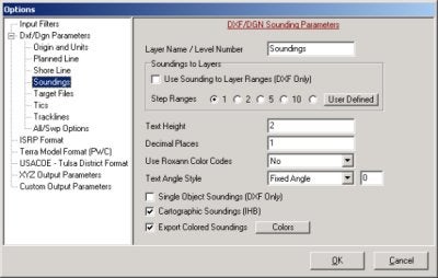
You can now export soundings to different layers and colors depending on ranges, export cartographic soundings, and even export single object soundings, whereas the old program created separate entities for the whole number, decimal point and decimal values. The color ranges are derived from the standard Hypack® Max color settings dialog box, like all the other color dependant programs.
Truncation and rounding rules are taken from Hypack® Max’s Control Panel. By selecting Truncate to Tenth (under the Soundings tab in the Control Panel), your DXF soundings will be lopped off to the tenth decimal place. By using the rounding rules, your soundings will be rounded to the user specified tenth, half or whole number.
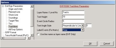
Added to the trackline export is the option to label events with either the event number or the event time. DXF export also gives the option to export each trackline to it’s own layer.
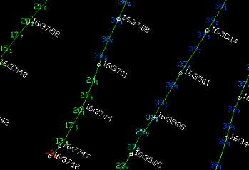
The example below shows the DXF file as displayed in AutoCAD. The soundings are truncated to the tenth decimal place, colored, cartographic style, and on different layers. The tracklines are exported with time labeled events, and each trackline is on it’s own layer.
Q水路設計(チャンネルデザイン)プログラムでの測線ファイル(*.lnw)の利用(Channel Design Center Line Import)[英語]
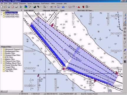
The change that was made to Channel Design was not driven by a customer request, but by a desire to provide an easier method of creating a channel file. You can now import a .LNW file, created using the centerline method in the Line Editor, into a Channel Plan file (*.PLN). This allows you to create a line file and clip it to a known channel. You can then quickly modify this into a Channel Plan file that includes template information for volumes calculations. The procedure is outlined below.
- Create a Line File using the centerline offset pattern in the Line Editor. I chose a BSB chart to provide my channel for this demonstration. The survey lines cover the area. You do need such tight line coverage to create a nice channel.
- Clip the lines to your channel using a Border file and the Clip Lines feature in the Line Editor.
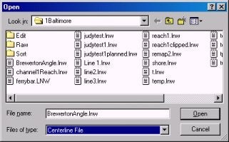
- Open the Line file you have just created in the Channel Design program. When the program reads the file, it uses the first line in the file as the centerline of our channel. Once the line is read, it behaves just like a normal plan file.
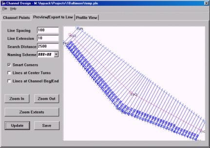
The start and end points of each line are used to create the left and right toes. Since there are more lines in the file than it requires to create the shape of the channel, the program eliminates points where three or more are in line with each other (using a one foot tolerance). This reduced the original 235 lines created in the Line Editor to 4 left toe points, 3 center line points and 2 right toe points.
Now we have defined the channel using the centerline file, but we do not have a line file with the template data yet.
- Edit depth, slope and chainage according to your channel. The defaults are:
- Depth: 20
- Slope: 3
- Chainage: 0
- Create a channel by clicking [Update]. In this example, I have used Smart Corners to fill the gap that we saw at the curve in the original line file. The channel created should have all of the correct settings with template information that can be used to compute volumes and we have coverage on the curve.
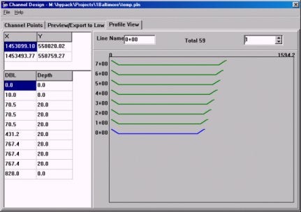
- Check your channel templates using the Profile View to make sure that all of the templates look good and that the channel was created correctly.
- Return to the Preview Tab and save your new Line File by clicking [Save] and naming your file.
Q水深データの処理(Sorting Elevation Data)
以前、同一週、同一エリア調査されたにもかかわらず、結果が大きく異なるデータがありました。
2つのデータはHypackのSortプログラムで並び替えられたXYZファイルです。これらのデータはSortプログラムの半径の設定を5フィートで並 び替えしたものです。Sortプログラムは設定された範囲内の最浅値を採用するようになっています。一般的にほとんどのデータではこの処理は問題なく動作 していました。
ただし、今回のデータでは少々手を加える必要がありました。
Hypackでは通常測深値をプラスの値として扱います。逆に標高値はマイナスとして扱っています。従って10mから20mの測深データを扱う場 合、Sortプログラムでは10mの測深値を採用します。しかし、-10mから-20mの測深データを扱う場合は-20mの値を採用します。従って、標高 データを扱っている場合は、標高データが全てプラスの値となるように変換しなければなりません。
つまり今回のデータは片方が測深値をプラスとして扱っており、もう一方が測深値をマイナスとして扱っていたために発生したものでした。
上記のような問題がありますのでSortプログラムを使用する場合は測深値の符号に注意してください。
Q複数の調査船の使用(Multiple Vessel Tracking in HYPACK® MAX)[英語]
I recently was asked by a customer how does a customer track multiple vessels on the screen in HYPACK MAX. I created a demonstration project to display two survey vessels and a dredge on one screen so that the operator can monitor the progress of all vessels.
When I was creating this demonstration I found a new use for a feature in Survey. By right clicking on a vessel you can assign that vessel to the Main Vessel. When you do this the survey screen will shift to always keep that vessel in the Map window.
To connect all of the vessels to one computer you need to have radio modems connected to each vessel to be monitored, and a modem connected to the monitor station for each vessel that will be tracked.
If there are several vessels to be monitored the monitor computer is going to need a serial port for each radio modem. Another key thing to remember is each radio modem pair must have a distinct frequency.
On the monitor computer the HYPACK Hardware program is configured with multiple NMEA devices and multiple mobiles ( one for each vessel ). In Survey you can then see each vessel on the screen as it moves independently from the other vessels. Only the main vessel can be used to record data. The data from other mobiles will be saved to files but those values will not be used to fill a matrix in Survey.
Qフィラデルフィア法体積計算2(Explanation of Philadelphia Volume Summaries)[英語]
I recently was asked by a user what all of the different items that were included in the Philadelphia Post-Dredge Volume Summary meant. It took me a couple of minutes to figure it out, even though I work with it about every other week. I figured it would be good to run a test example and explain some of the output.
Step 1: 8.5m Data Set in Philadelphia Pre-Dredge
I first created two test data sets that would create a set of data at 8.5m and 9.5m across my survey lines.
My first data set and the associated cross section template are shown in the figure to the right.
The template points are as follows:
| Distance | Depth |
|---|---|
| 0.0 | 0.0 |
| 50.0 | 10.0 |
| 100.0 | 10.0 (Centerline) |
| 150.0 | 10.0 |
| 200.0 | 0.0 |
All of the depths in the first data set are at 8.5m. There are ten parallel lines.
I first ran the volumes for this data set using the Philadelphia Pre-Dredge method. This generated the report shown to the right:

The Left Slope and Right Slope areas are reported as 5.63 m2each. This is correct as shown in the figure below.
The area for the Left Channel and Right Channel is simply the height times width (1.5 x 50) and the 75 m2 shown in the report is correct.
Since each section is identical, the volume is equal to the sum of the area under each section (161.25² ) multiplied by the distance between sections (100) giving 16125.00 m³.
The overdepth template was placed one meter below the design template. The results from the volume report are shown in the figure right.
The left slope area is identical to the right slope area and is shown in the figure below. The volume is shown to be 10m², which is identical to that shown in the CROSS SECTIONS report.
The overdepth in the Left Channel and Right Channel is equal to the depth of overdepth template beneath the design template (1.0m) times the distance (50m) which is 50m².
The area between two sections is equal to the average area under a section (120m; they are identical sections) times the distance between sections (100) resulting in 12,000 m³ which is the volume shown in the report.
The results for the channel (nine pairs of lines) are shown in the figure to the right.
The Total Material To Project Depth is total volume of material located above the design template. This is equal to our area per section above the design template (16,125 m³) times the number of pairs of lines (9) and is exactly correct.
The Total Allowable Overdepth is the total amount of material located between the design and overdepth templates. This is equal to our volume per section (12,000 m³) times the number of line pairs (9) = 108,000 m³. Once again, the CROSS SECTIONS program is exactly correct.
The Total Pay Place is simply the sum of the two items above.
Step 2: 9.5m Data Set in Philadelphia Pre-Dredge
I next created a new data set, using the same template, but changing all of the depths to 9.5m. A typical section is shown in the figure right.
The design material is shown in the figure right. I’ll leave it to you to prove the areas and volumes are correct. [Trust me, they are.]
The overdepth material is shown in the figure right. Once again, feel free to verify that the areas and volumes are correct. [They are.]
Finally, the volume summary from the Philadelphia Pre-Dredge report is shown in the figure to the right. All values are correct and now we are ready for the BIG test.
Step 3: 8.5m and 9.5m Datasets in Philadelphia Post-Dredge Method.
Finally, I entered both the 8.5m dataset (PreDredge) and my 9.5m dataset (PostDredge) datasets into the Philadelphia Post-Dredge Method and examined the results. A typical cross section is shown in the figure right.
Notice that the program now colors the material removed, not the material remaining. This is something that confuses a lot of users.
The results for the first two sections are shown in the figure to the right.
The “Area” shown in the report is the area of material removed in that section. Note that it is possible to get a negative area for a segment if the area computed from your post-dredge survey is greater than the area from your pre-dredge survey.
| Left Slope | Left Channel | Right Channel | Right Slope | |
|---|---|---|---|---|
| 8.5m Area | 5.63 m² | 75.00 m² | 75.00 m² | 5.63 m² |
| 9.5m Area | 0.63 m² | 50.00 m² | 50.00 m² | 0.63 m² |
| Material Removed | 5.00 m² | 25.00 m² | 25.00 m² | 5.00 m² |
The Remain areas are generated from the 9.5m data set and are identical to those computed when we ran the Philadelphia Pre-Dredge volumes for that data set.
The volume for the first section (11,000 m³) is the same value achieved by taking the volume for the 8.5m data set (16,125 m³) and subtracting the volume from the 9.5m data set (5,125 m³). The same is true for the Overdepth areas and volumes.
The summary for the Philadelphia Post-Dredge Volume Report is shown above. The values are explained as follows:
Total Removed To Project Depth: This is the difference between the volume (above design template) computed for the Pre-Dredge data set (145,125 m³) minus the volume computed for the Post-Dredge data set (46,125 m³). Note that this can be a negative number if there is more material present in the Post-Dredge survey!
Total Pay Removed in Overdepth: This is the difference between the volume of material contained in the area between the design and overdepth templates for the Pre-Dredge data set (108,000 m³) minus the volume for the same area in the Post-Dredge data set (99,000 m³).
Total Pay Removed: This is the sum of the Total Removed to Project Depth and the Total Pay Removed in Overdepth.
Total Removed: This is the total material difference between the Pre-Dredge survey and the Post-Dredge survey without regard to the design and overdepth template. In our example, the survey area covered a 200m x 900m area (180,000 m²). We changed the surface from 8.5m to 9.5m, taking away 1m of material. Multiplying the area (180,000 m²) by the height (1m) gives us 180,000 m³, representing the Total Removed.
Total Remaining Above Project Depth: This is the remaining material above the design template from our Post-Dredge survey. It is independent from the Pre-Dredge survey surface and represents how much material you have to remove to get the channel down to the project design.
Total Overdredged Material: This represents the material that has been removed beneath the overdepth template. It is computed by taking the Total Removed (180,000 m³) and subtracting from it the Total Pay Removed (108,000 m³). In our example, this results in an answer of 72,000 m³.
Total Infill Material: This is the volume of material where the Post-Dredge survey is deeper than the Pre-Dredge survey. In our example, we have no such area and the result is 0.00 m³.
Q水路設計(チャンネルデザイン)プログラムにおける急な変化を含むトウラインの処理(Channel Design with Sharp Turns in the Toe Lines)[英語]
A client recently had trouble creating an LNW file using the CHANNEL DESIGN program. The problem end of the channel is shown in the figure to the right.
The Left Toe line is shown at the top of the figure in blue, with points 2L, 3L and 4L being visible. There is a 90º turn at each point.
When the planned lines were generated in the CHANNEL DESIGN program, the result is shown in the figure right.
At first glance, it appears that lines 8+80, 9+00 and 9+20 have been extended too far from the left toe line and are erroneous.
It turns out the CHANNEL DESIGN is doing a pretty good job in this case! Take a look at the figure to the right.
One of the first things that CHANNEL DESIGN does is to construct the Left and Right "Top of Bank" lines. These are constructed from the positions of the toe lines and the side slope information. The Left Top of Bank line is shown in red at the top of the figure.
CHANNEL DESIGN is smart enough to be able to handle the 90º turns and generate the correct top of bank line.
For each planned line, the program then checks to see where it crosses the "toe line" and where it crosses the "top of bank" line.
As a test, I changed the Side Slope on the left side of the channel from "2" to "0.5". This would result in a "steeper" bank and the Top of Bank line should be generated closer to the Left Toe Line, eliminating the "long" lines at the end of the channel.
The figure to the right shows the result, confirming the fact that CHANNEL DESIGN is working as designed in this case.
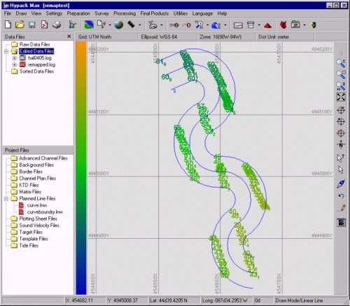
Qリマッププログラムが曲線を含んだ測線の処理が可能に(Curved Lines Added to Re-map)
Remapプログラムが曲線を含んだファイルに対応しました。RemapプログラムはHYPACK® All FormatファイルからASCII xyzファイルを作成またはHYPACK® All Formatファイルを再作成するユーティリティーです。測深値は選択されたラインに従い任意の位置に出力することが可能です。
以下に示された図は、センターラインより左右に25feet離れた位置に1本ずつ測線が描かれている例です。
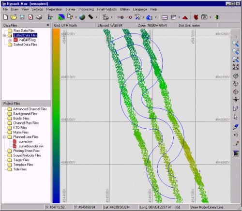
Re-mapプログラムを以下の設定にて実行します。
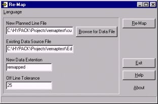
結果は以下の通りとなります。
Qシングルビームエディターにおけるビームステアリング(Beam Steering in the Single Beam Editor)[英語]
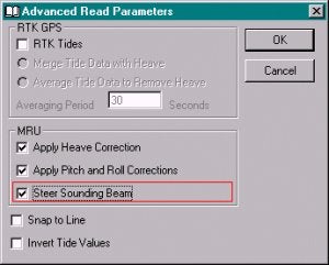
The beam steering option in the single beam editor controls the depth and location of Hypack® soundings. The default setting is off (do not steer the beam), which is correct for most installations. There are certain circumstances where beam steering is desirable, which of course is why we put it in the program.
What is beam steering? It is the aiming of the sounding beam in the direction given by the pitch and roll sensor. Just like a flashlight. If you do not have a pitch and roll sensor, obviously you do not want beam steering. If you have a wide angle transducer, you still do not want beam steering (for less obvious reasons described below). If you have a narrow beam transducer, a pitch / roll sensor and you work in rough water, you may want to steer the beam.
First, we look at a sounding taken in calm water over a relatively flat bottom. Narrow beam or wide beam, beam steering or not, sounding depth and location will be the same and correct.
Next we look at a sounding taken in calm water on a steep slope. The echosounder returns a depth corresponding to the first return, which in this case is not directly under the transducer. Note that the error increases with beam width, which is a good argument for using a narrow beam transducer.
(Methods exist to "migrate" the sounding to it's proper depth and location but to my knowledge, no one uses them.)
In the two examples above, beam steering has not been an issue because the beam is close to vertical. Now we examine a few cases where the beam is not vertical, i.e., pitch and roll angles are involved.
The first diagram to the left shows the case of the wide beam transducer. The depth returned from the echosounder is the true depth directly beneath the transducer. It will be recorded properly by Hypack® when beam steering is off. If beam steering is on, it will be recorded forward and slightly shallower than actual. Moral is: don't use beam steering with wide angle transducers.
The final example shows a narrow beam pitched forward. The actual sounding point is the closest bottom point within the cone of sound. Note that the sounding point calculated without beam steering is slightly off as is the sounding point calculated with beam steering!
This is getting complicated, but at least one thing is clear: when the combined pitch and roll angle is less than the beam width, do not use beam steering. I think this covers all protected water surveys, regardless of beam width. For open water surveys, consider beam steering when the boat attitude angle is much greater than the beam width. If the boat is rolling +/- 10 degrees with a 3 degree transducer, definitely consider beam steering.
Qシングルビームデータと体積計算について(The Effect of "Along-Line" Spacing of Soundings in Single Beam Data on the Computation of Average End Area Volumes)[英語]tion of Average End Area Volumes
Well, that's a hell of an impressive title. If I were to tell you of a way that you could make $20,000 without any additional effort would you be interested? If I tell you how, would you give me half? If your answer to the last two questions is "Yes", then read on. Otherwise, go look at the cartoon.
HYPACK® can collect every sounding that comes out of your echosounder. If your sounder is updating at 15 times per second and your boat is traveling at six knots, this means you will have a sounding every 8" along your planned line.
Now, when you go to compute volumes, should you use all of these soundings or should you "thin" the data by using one of the sounding selection programs?
In preparation for my Volume Seminar at the 2001 U.S. Hydrographic Conference (21-24 May 2001 - Sheraton Norfolk Waterside Hotel - details at www.thsoa.org) I took a single beam data set and did some tests to determine how the volumes compared when I thinned the data using different spacings.
Below is a plot, taken from a capture of the CROSS SECTIONS program. The original survey data is spaced about every 8" and is in black. I then ran the data through the MAPPER program, using a 20' x 20' matrix and saved the point "Closest to the Center" of each cell to an XYZ file. [It's a little more complex, as I then took the XYZ file result from MAPPER, ran it into the TIN MODEL and then cut sections through it to get it back into EDITED ALL format so I could then load the results back into CROSS SECTIONS.] The soundings at 20' spacing are shown in red on the picture below.
Visually, there isn't a whole lot of difference between the two sections. The file with the 8" spacing moves above and below the file with the 20' spacing, but it's not evident what the effect will be on the volumes.
I ran volume quantities for the entire channel, once for the 8" data and again for the 20' data. The 8" data had almost 3% more material. I then ran some more tests, sampling the data at 2', 5', 10', 20' and 50' spacing to see the result. The computed volumes are summarized in the table and graph below.
| Spacing | Dredge Material (cubic yards) |
% of original |
|---|---|---|
| 8" | 28,938 | 100 |
| 2' | 28,911 | 99.9 |
| 5' | 28,782 | 99.5 |
| 10' | 28,009 | 96.8 |
| 20' | 28,151 | 97.3 |
| 50' | 28,630 | 98.9 |
The test conducted on this data set was repeated on a different data set with almost identical results.
So, if I want to maximize my volume quantities, I will use every data point in the sounding set. If I want to minimize my volume quantities, I will thin the data every 10' along the line.
The difference in this data set between those two approaches is 929 cubic yards. At $22/yard, that comes to a savings of $20,438.
Q複雑な調査船の作成
最新のBoat Shape Editorでは複合的なボート形状を作成することができます。そして、Surveyプログラムにおいて作成したボートを表示することができます。そし て、作成したボートの色とラインカラーを指定することができます。また、どこでそれらのアンカーが位置しているかを示すアンカーポイントを設定することも 可能です。設定したアンカーは、Surveyプログラムで表示することができます。
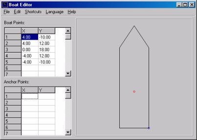
例として戦艦USSワシントンのボート形状を作成しました。まず、ボートの各折点の座標を得るために、戦艦のダイアグラムをディジタル化します。それから船の一般的なアウトラインのポイントを入力します。ボート起点( 0X、0Y )を適当な位置に設定し、その周辺でアウトラインを作成します。基点より右舷側がXの正方向、前方がYの正方向です。
次のステップは、戦艦の特徴(ブリッジ、銃、スタック等)のそれぞれの座標値をDrawing Objects欄に入力します。これらの座標値は、1つのラインとして入力されなければなりません。この戦艦上の砲台などに独立した動きなど加える場合、 対象となるオブジェクトを別の船として登録します。そうすることでSurveyプログラム上に回転する砲台などを表示することが可能になります。
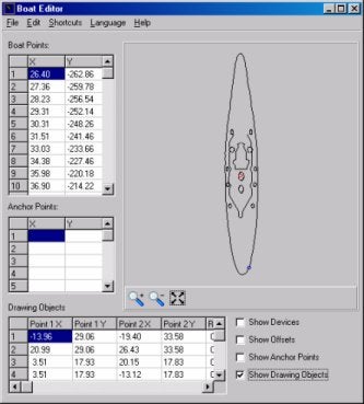
以下にHYPACK® Surveyで表示された戦艦を示します。砲台を回転させるにはHYPACK® Hardwareでsim32.dllのコントロールパネルで設定します。
sim32.dll (海岸のOceanographics Generic Simulator )は全ての移動体のヘディングデバイスとして使用することができます。
下記に揚げる例はF18と航空母艦です。
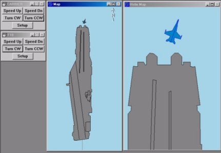
これらの例はHYPACKにおける可能性を示すデモンストレーションデータです。
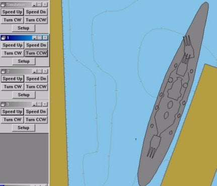
次のイメージは、Boat Shape Editorで多く望まれている例です。この例は、Surveyプログラムで表示されているように、浚渫機の右舷にサイド艀がある浚渫機形状を示しています。
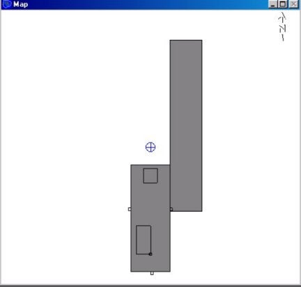
メインアウトラインは、Boat Shape EditorにおけるBoat Pointsとして、小鋤、クレーン等のような他のアイテムはDrawing Objectsとして作成しています。サークル記号は、Hardwareにおける第2の船として加えられたバケットのポジションである。
これらのボート形状は、HYPACKでは*.shpファイルしてセーブされます。(あらゆるテキストエディタにおいて修正され得る、もしくは作成され得るシンプルなASCIIテキストファイルです)。
QNew Line Editor in Hypack ® Max 02.12a
The Line Editor has been redesigned recently and has been implemented in the new 02.12a release. Some of the new features include easy access to different lines within the *.LNW file, editing of templates and even creation of templates within the editor. The figure below shows a comparison between the old Line Editor on top and the New Line Editor at the bottom.
The buttons have been replaced with icons. Simply move the curser over each icon to display a description. The new Line Editor also displays all the line names/numbers in the left panel of the editor, making it easier to display the coordinates of a line by simply highlighting the line name or number. In the old Line Editor, you had to scroll through each line with an arrow key – pretty tedious if you have a line file containing a few hundred lines!
A brand new option is the ability to edit template information. This really comes in handy with line files created in Channel Design. Just open your *.LNW file in the Line Editor and highlight a line name/number in the left panel. Then go to the Template menu item and click on Edit. You’ll get the window shown below:
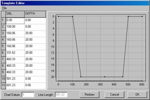
What you see on the left of the window are the template points, DBL (distance from the start of line in survey units) and depth. Change the DBL and/or depth and click on the Redraw button. The graph will then be updated with the new template points. You can modify each template separately, or apply the template changes to all the lines within that LNW file.
You can also create templates for 2D LNW files that were originally created in the Line Editor. These line files that can then be saved as 3D LNW files. This comes in really handy when you need to create a simple channel and all you have is a standard LNW file.