FAQ
FAQ検索結果
検索キーワード:
Q浚渫船の表示機能について(Dredgepack Shapes in the Profile Screen)[英語]
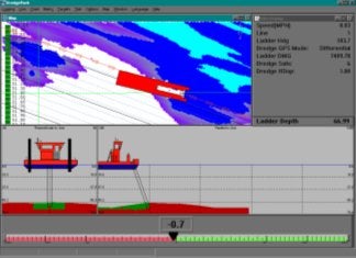
A recent development in Dredgepack is the ability to show the shape of the vessel in the Profile window. This image (right) was captured during a recent visit to the Dredge George McWallace. There are several items displayed here. In the Profile there are two sections. The section to the left is the view looking forward through the dredge. The arm of the suction is displayed. In this case the suction was a 30 foot wide dustpan dredge. The section to the right is the view looking across the path of the dredge or perpendicular to the vessel. In the perpendicular view the operator has the ability to see what material is ahead of the dredge.
The distance that is viewed in these windows are set by the operator in the Profile window setup menu.
In the next image we have a Degroot Cutter Dredger CZ 400. The plan of the dredge was scanned and forwarded to Coastal Oceanographics. The image was taken and cleaned so that small details are removed. This is because in a large drawing a small detail is nice but when the image is reduced to the size drawn below, the detail makes the image appear blurred. As the image below shows, enough detail was left to make the dredge readily identifiable to anyone that has worked on this type of dredge.
Also the plans of an Ellicot 370 were sent as part of a current project. This is the image from the Ellicot dredge. Most of the detail is removed to make the image appear clean and then colored in to enhance the display.
To change the image that is displayed in the Profile window the user is required to modify a configuration file. Configuration files are also known as ini files. This should sound familiar to anyone that has used an earlier version of HYPACK®. HYPACK® Max 2.12 includes a shapes folder where the BMP images and the associated configuration files are stored. Included in the shapes folder are images for the Default shape, Degroot dredge and an Ellicot 370. The current version of Dredgepack supports several items in the Profile window for the differing types of dredges. It is possible to show the Cutter Suction, Hopper Left, Hopper Center and Hopper Right. For every mobile with depth the user has a Profile window. That is why there are so many Hopper displays.
The next display is the Profile setup. The items on this display have been highlighted to show what applies to the Profile view.
The Paintshop Pro program was used to modify the shape image. Any graphics program that works with bitmaps can be used. The nice part of Paintshop is that the actual pixel position of the cursor is displayed. This is important for modifying the configuration settings.
A sample of the data that is stored in the configuration file is shown below. This data is modified to properly display the shape in the window. The same data is in the configuration file for the perpendicular and forward looking files. The file to modify the perpendicular view is the …prof.ini file and the forward view is the …cross.ini file. The "…" should be the cutter or hopper as the case may be.
Level is the water level on the image. This is where 0 will be.
Arm X is the distance from the left edge of the bitmap in pixels to the point the arm attaches.
Arm Y is the distance from the top edge of the bitmap in pixels to the point the arm attaches.
BMPFile is the image to display.
By modifying these items the Profile window can be adjusted to display a custom shape corresponding to any dredge.
[General]
LEVEL=120
ARMX=280
ARMY=120
BMPFILE=c:\hypack\shapes\Degrootprof.bmp
QシングルビームエディターにおけるRTK-GPS潮位データの処理(Elevation Mode and RTK Tides in the Single Beam Editor)[英語]
Recently, we had an situation where one of our users was using RTK (Real Time Kinematic) tide corrections while processing their survey data in elevation mode. When the data was read into the Single Beam Editor, the calculations were incorrect.
With closer examination of the measurements and the calculations that occur, we determined that when you convert single beam data to elevation mode and are using RTK tide corrections, an additional adjustment is required. The tide correction value must be negated.
Let's take a closer look.
Most surveys are done in Depth Mode where the sounding depths are positive values. In Hypack® Max, the tide correction value is added to the sounding depth to remove the effects of the change in tide. Since we want to remove this amount from the sounding depths, the value must be negative. [C = A + (-B)]
For example:
Where A = 30, B = 5, C = 25, the equation becomes 25 = 30 + (-5).
In Elevation Mode, the sounding depths are negative. The tide corrections, therefore, must be positive. Using the example above, the equation becomes -25 = -30 + 5.
For Single Beam surveys:
- Convert the Depths to Elevation Mode by selecting Depths--Invert Only in the Read Parameters dialog.
- Convert the tide correction from negative to positive by checking the Invert Tide Values box in the Advanced Read Parameters dialog in the Single Beam Editor.
For Multibeam surveys all corrections are automatically adjusted by the Hysweep Editor without further action by you.
QMBMaxフィルタ機能(Multibeam Max Sounding Filters)
MB-MAXマルチ‐ビーム処理プログラムには、未編集の調査データをクリアにするためにいくつかのフィルタ機能があります。それらのフィルタは、最小の、そして最大の深さのような非常にシンプルなフィルタから、洗練された統計処理のフィルタまで多種多様となっています。
一般的なフィルタ(General)
下図のスクリーンキャプチャは、Mbmaxで利用可能な一般的なフィルタオプションを示しています。
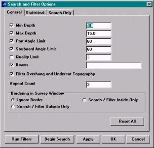
- Minimum and Maximum Depth:調査エリアにおける既知の情報から最大水深、最少水深を設定します。
- Port and Starboard Angle Limits:有効とするビーム角を設定します。
- Quality Limit: マルチ‐ビームソーナシステムによって出力される品質コードに基づくフィルタリング行います。
- BBeams: 不正確であることが既知であるビームに対するフィルタです。
- Filter Overhang and Undercut Topography: オーバーハング、または、アンダカットに現れるあらゆる地形の特徴を考慮してろデータの排除を行います。全てのこの種類のほとんどの地形は音響エラーによるため、ソフトな底質をもつエリアでは非常に効果的なフィルタとなります。
隣接しているオプションは、フィルタの範囲を設定するために使用します。
統計的フィルタ(Statistical)
水深データがFill Matrixによってグリッド化された後に統計的フィルタは、有効となります。グリッド化は、比較処理をする測深データポイントを集めるために必要となり ます。-その統計は、個々のマトリックスセルで計算されます。それらのオプションは、下図のスクリーンキャプチャにおいて示されます。:
セル統計値(Cell Statistic):
MB-Maxユーザーは、5種類のセル統計フィルタを選択できます。
- Maximum: 最深値
- Minimum: 最浅値
- Average: 平均値
- Median: 中間値
- Mode: 最頻値
Median、及び、Modeは、最も有効な手段です。Averageは平均を崩すような他の残りの測深データのうちの1つがはるか遠くにあるようなセルを除いて有効な手段となりえます。
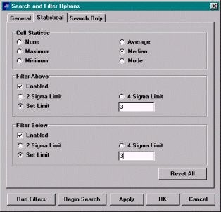
Filter Above and Below:
上記で選択された統計方法の許容範囲をセットします。例えば、MedianがCell Statisticで選択され、そして、上の制限が3に設定されている場合、平均深度からそれから、3フィート/メータ以上の測深データは排除されます。
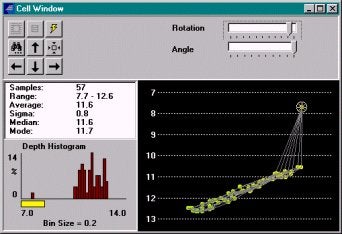
セルウィンドウ
セルウィンドウ(下図)は、アクティブフィルタ、及び、セルの統計的特性をグラフィカルに表示します。下記の例のように、統計の限界を越える1つのポイントは、測深グラフ(黄色のX )、測深ヒストグラム(黄色のバンド)で強調されます。双方の画面において、測深エラーは、真の水深データから離れて存在しています。
検索とフィルタ
1つのマウスクリックで一連のデータセットをクリーニングすることは非常に魅力的です。しかし、実際上、難しいことです。問題は、良い水深データを保持しながらも、エラーを取り除くことです。
Mbmaxは、この問題を検索機能によって解決します。: generalとstatisticalを設定し、Begin Searchボタンをクリックします。プログラムは、水深データをスキャンし、フィルターで設定された範囲を超える最初のポイントを黄色のXマークで表示 します。その後、オペレーターはそのデータを取り除くか、保持するかどうか決定します。Filterボタンをクリックすると、水深データは取り除かれま す。Find Nextボタンは、それを保持して次の該当データを捜します。この処理は少々時間を要しますが、各ポイントが除去の前に検査される利点があります。
Qパッチテストの”不確からしさ”について(Patch Test Uncertainty III)
GPSポジションエラーがヨーテストに与える影響について説明します。
ヨーテストは様々な地形エリアで行います。同方向の測線を走行します。測線間隔は十分なオーバーラップができるようにするため、そのエリアの深さによって異なります。
ヨーとポジションエラーの関係は以下の式によって与えられます。
f = tan-1 ( dp / z )
f :パッチテストの結果
dp :ポジションエラー
z :水深値
ヨーとポジションエラーの関係
| Case | Water Depth (feet) | Position Error (feet) | Yaw Bias (+/- degrees) |
|---|---|---|---|
| 1 | 300' | 6' | 1.1 |
| 2 | 100' | 6' | 3.4 |
| 3 | 40' | 6' | 8.5 |
| 4 | 40' | 3' | 4.3 |
| 5 | 40' | 1' | 1.4 |
| 6 | 20' | 6' | 16.6 |
| 7 | 20' | 3' | 8.5 |
| 8 | 20' | 1' | 2.7 |
QAlert! Hyplot Max, Windows 2000 and HP DesignJet Plotters![英語]
We have recently come across an issue concerning Hyplot Max under Windows 2000. This only seems to happen when plotting to HP DesignJet printers.
You may get a General Protection Fault when trying to plot from Hyplot Max to a DesignJet plotter. This seems to happen after you choose the plotter from the Windows Printer dialog and you click the Print button. This may cause your computer to reboot all of a sudden.
While we are still looking for the source of the problem, there is a way around the problem. Once you click the Plot button and select your HP plotter, click on the Properties button. Go to the Advanced tab and click on the In Computer button (see figure below).
Click OK, and then click the Print button. You should then be able to plot from Hyplot Max on a Windows 2000 PC to an HP DesignJet without a problem.
QHypackMAX2.12インストールに関する注意[英語]
When we send out an entirely new release to our clients who are active on the maintenance plan, it’s our hope that at least the majority of you make the transition to the new version. Philosophically speaking, we view each release as a unit. All of the parts contained within are carefully balanced and have been tested together as a group. So we recommend that you do not install a new version on top of an older version. You can probably get away with it, but there are several instances where it may cause havoc. We suggest you either “uninstall” Hypack via the normal windows way (this will not uninstall any projects) or rename the folder of the older program to C:\Hypack_old and install the new version to the standard c:\Hypack folder. If you use the latter method you will then have to move your projects back to the c:\Hypack folder manually.
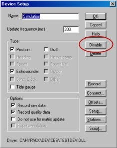
New Feature in Hardware Coming in 2.12A
The “disable” button makes its way to the new release. Time was that you had to got through the drudgery of deleting one device at a time if you had some sort of communications port conflict. Then you had to go through the whole reloading process, adding a new driver back again, after you caught the conflict.
Lets say you switch between many devices. Now you can keep them all in one hardware setup and “disable” or “enable” them as they come on/off line.
Qサーベイプログラムの自動処理(Procedure for Automatically Starting the Survey Program)[英語]
This procedure is intended to allow a user to configure a project in the HYPACK MAX software and then start recording position data automatically without any user intervention. This is to recover from a loss of power and start logging data as soon as the computer is restarted. It was originally devised for a customer who wanted to set up three RTK-GPS receivers on a building to monitor movement during an earthquake. Because of the risk of loss of power, this procedure necessitated the startup and logging of data within the Survey program as soon as the PC was booted up.
The first requirement is that the user has configured a project with the parameters and names for that project. In this demonstration, I named the project Hong Kong. The Geodetic Parameters and Hardware must be configured as you would in any Hypack project.
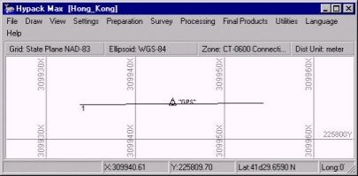
The project must have a Planned Line file. All you really need is a single short line to automatically log data upon entering Survey. For a stationary GPS, you should create this line as short as possible and as close to the GPS antenna position as possible. In this demonstration, I created a single planned line 20 meters long. The GPS antenna was situated around the centerpoint of the line file as shown below.
Survey's Start Line Gate must be set to a value greater than the distance from the antenna to the line file. In order to log automatically upon entering Survey, the Start Line Gate should be greater than the line length. In this case, the line length is only 20 meters. I set the Start Line Gate to 100. This will allow the program to automatically start logging when the program is started.
To set the Start line gate the user must enter the Survey program and modify the Navigation Parameters. Once this is set the user cannot exit Survey without resetting this to zero because the Survey program will not allow the user to exit without stopping logging. The program will continue to restart the logging function as long as the GPS is within the start line gate distance. The Navigation Parameters are shown below.
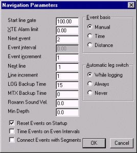
Another parameter that should be set is the Log Backup Time. This is also set in the Navigation Parameters. This should be set to an interval consistent with the project requirements. This configures the software to close the datafile after the predetermined period and start a new datafile. You will notice I set the LOG Backup Time to 15. Survey will close a datafile and open a new file every 15 minutes. This keeps files much smaller, and in the case of loss of power, computer crash, etc., only 15 minutes of data would be lost, rather than a whole day's worth.
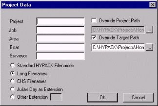
If LOG Backup time is used, Long Filenames should be selected in the Project Information menu of the Survey program as shown below.
The next Item to create is the shortcut. This is done in either Windows Explorer or by selecting the drive through My Computer. Find the Survey32.EXE program in the HYPACK folder on your computer.
The user can then create a shortcut to the Survey32 program by right clicking on survey32.exe, and then clicking on Create Shortcut.
Next we have to Edit the Shortcut. Right click on the shortcut. On the menu that appears the user should select the Properties menu item.
To modify this the Target parameter should be modified. The correct method of launching a program is to add the project and project.ini to the path.
Example: C:\HYPACK\survey32.exe /pProjectName /iProjectName.ini
In this example, the target should look like this:
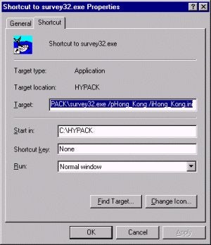
C:\HYPACK\survey32.exe /pHong_Kong /iHong_Kong.ini
The last step in the procedure is to add this shortcut to the Start Menu. This shortcut must be added to the Startup item on the Start Menu to allow the program to automatically start when Windows boots up. You can do this in Windows Explorer. Just drag this shortcut into the \Windows\Start Menu\Programs\StartUp directory as shown below.
Once these steps have been completed the user will have a system that automatically recovers from a loss of power and restarts Survey. It will also automatically start logging data upon reboot.
Q曳航体用ケーブルドライバの使用報告(Towcable.dll -- A Report from the Field)
Tow cableドライバは曳航器のより正確な位置計算を可能とするドライバです。このドライバは何人かの客先でテストし、MYPACK Maxを用いたより良い曳航器のトラッキング理論として完成しました。
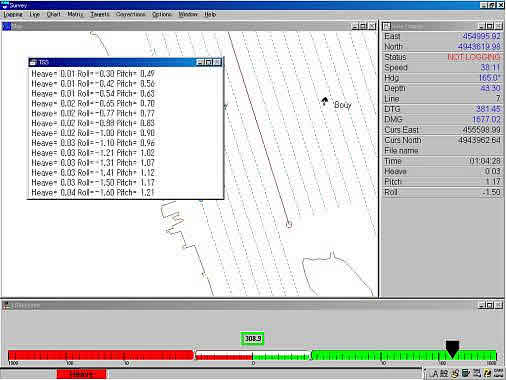
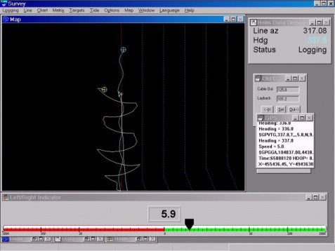
下記の例は実際のテスト結果です。この図によりトラッキング性能が分かると思います。
上の図で青い線は船の位置で、赤い線が方位を用いて計算された曳航器の位置です。このテスト、及び他の幾つかのテストによりこの理論が曳航器の位置計算に最も適していると言えるでしょう。
HYPACK Maxで2つのラインを画面上に同時に表示するためには以下の手順を踏んでください。
- まずHYPACK MaxのCONTROL PANELを開いてください。これはSETTINGメニューからCONTROL PANELを選択、または鐫と金槌のアイコンをクリックしてください。
- タブからTrack Linesを選んで下さい。イメージは以下の図のとおりです。
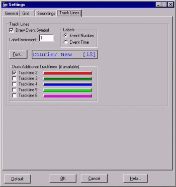
- ここでユーザ側が全てのトラックラインについて、表示、非表示等の変更を行えます。それぞれのトラックラインの色は変えることが出来ませんが、Main Vesselの色のみ、Fontボタンで変えることができます。
QJacksonville法体積計算(Modification of Jacksonville Post-dredge Method to Compute Boxcuts)[英語]
Fran Woodward of the USACE Jacksonville District recently got in touch with us and requested some changes in the Jacksonville Post-dredge computation method that currently exists in the CROSS SECTIONS program. These changes include:
- The ability to compute the overdepth material using either ALL or Contour dredging methods.
- The ability to exclude the side slope areas from all computations.
- The ability to compute box cuts that provide for side slope material to slough off into voids created beneath the overdepth template around the toes.
There are now two options for the computation of overdepth material. These are "All" and "Contour". Using the "All" option, all material in the area between the design template and overdepth template will be computed. Using the "Contour" option, overdepth material will only be computed where the measured depth is less than the design template. This is identical to the technique used in the Philadelphia Methods of CROSS SECTIONS and the TIN MODEL.
The big change is the revised computation of box cut quantities. Take a look at the figure.
Digging precisely on the side slope is a hard job. In areas where the bottom material is soft, contractors are sometimes allowed to dig deep holes at the toe locations, with the idea that the material on the side slope will fall into the holes created.
In a soon-to-be released version of the CROSS SECTIONS program (it didn't make the 00.5B release), the following quantities will be computed separately for the left side and right side of each pair of survey lines.
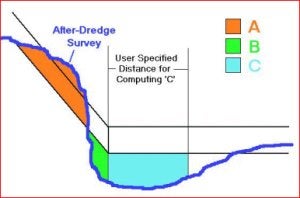
A =The remaining side slope material from the after-dredge survey that is above the overdepth template. This will include all material above the design template and between the design and overdepth templates. This material is orange in the above figure.
B =The void present from the toe line outward from the centerline where the after-dredge survey is deeper than the overdepth template. This material is green in the above figure.
C =The void present from the toe line inward towards the centerline a user-specified distance where the after-dredge survey is deeper than the overdepth template.
These areas are computed for each line. [Separate areas are computed for the left and right sides of the channel. The program then uses the Average End Area formula to compute the volume of material contained in the A, B, and C areas between each pair of survey lines.
The Box Cut Volume is then determined by using the following rule:
If A > (B + C) then Box Cut Volume = B + C
If A < (B + C) then Box Cut Volume = A
For example, if I have 80 yd³ of available material remaining on the side slope and I have dug a void of 200 yd³, I'm only going to get credited 80 yd³. [I can't have more material fall into the hole than actually exists.]
Likewise, if I have 150 yd³ of available material on the side slope and I have dug a void of 75 yd³, I'm only going to get credited 75 yd³. I'm only going to get credit until the void is full.
QSurveyプログラムのWindowメニューでTSSのデータを確認すると正しく来ているのに画面下に"Heave"と赤く表示されるのはなぜでしょう?
HYPACKを終了し、DMSView又はターミナルソフトを使用してTSSからのデータを見て下さい。
データ中に含まれているフラグが小文字になっていませんか?(下図参照)
これは、何らかの原因でセルフテスト実行中である事が考えられるので大文字の"U"になった後に測量(Survey)を開始して下さい。
| 023DE7-0007u 0023 | 0038 |
|---|---|
| 023DF6-0007u 0016 | 0041 |
| 053E1C-0007u 0009 | 0044 |
Q新測地系(WGS-84楕円体)への対応
図1を参考にGeodetic parameters(測地パラメータ)の設定を行なって下さい。
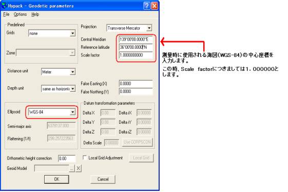
図1.WGS-84楕円体使用時の設定
参考:GRS80楕円体を使用する時
図2を参考にGeodetic parameters(測地パラメータ)の設定を行なって下さい。
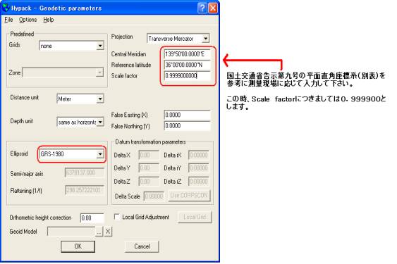
図2.GRP80楕円体使用時の設定
Qマルチビームパフォーマンステスト(Multibeam Performance Testing)
このプログラムはマルチビーム測深機の精度を検証する際の参照用プログラムです。HYSWEEP Survey プログラムまたはMultiBeam Maxにて使用することができます。
以下に使用法でマルチビーム測深機の様々なテストを行うことができます。
バーチェック:
バーがマルチビームのどのビームに位置しているかを特定することが難しいことと、複数のビームがバーで反射するため、従来シングルビーム測深機で行われて いたバーチェックをマルチビーム測深機で実行することは困難です。そこで、一定時間にバーにあたる全ビームの平均値を結果とします。 測深とビームアングルゲートを使用して海底やバーをつるしているチェーンの影響を除くことができます。
マルチビーム動作確認
非常にシンプルなテスト方法を紹介します。まず、非常に狭い平坦なエリアを200パーセントのカバレッジで往復します。この調査では編集、グリッド化、平 均化したデータをリファレンスとして使用します。次にリファレンスを作成する際に使用した測線と直行するように1往復の測線を走行し、リファレンスとの差 を比較します。
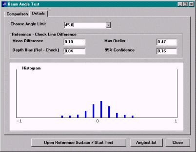
計算された統計値はリファレンスラインとの比較を示します。
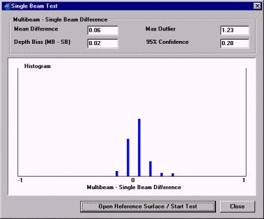
シングルビームとの比較
シングルビームとの比較は、上述のようにマルチビーム測深機で作成したリファレンス上をシングルビームで再度走行することで行います。
QXYZデータファイルの結合(Merging XYZ Data Files)
2つのXYZファイルを結合するには、エディター上で結合する若しくはDOSコマンドで以下の様に入力することで簡単に実行できます。
copy file1.xyz+file2.xyz file3.xyz.
通常はこの方法で十分な結果が得られるでしょう。
浚渫後の地形ファイルであるfile2.xyzのエリアが浚渫前の地形ファイルであるfile1.xyzのエリアより狭い場合、通常必要なデータは file2.xyzのエリアのみ置きかえられたXYZファイルを作成することでしょう。この値を全自動で計算する方法はHypackには存在しません。 Hypackでこの値を求めるには以下の手順を実行することで可能です。
- file1.xyzファイルをプロジェクトに読み込みます。
- Border editorを使用してfile file1.brdファイルを作成します。このとき境界線を構成する点の最後の点を囲みたいエリアの外に設定します。
- file1.xyz上で右クリックし、Clip to Borderを選択し、file1.brdファイルでデータをクリップします。
- file2.xyzをプロジェクトに読み込みます。
- Border editorでfile1.brdファイルを読み込み、最後の点を、囲みたいエリアの内側に設定し直して、再度.file2.brdとして保存します。
- file1.xyzと同様にクリップされたファイルを作成します。
- 上記手順で作成した2つのファイルを結合することで浚渫エリアの測深データのみが置きかえられたXYZファイルが作成できます。Tinモデルプログラムを使用して上記と同様なことを実行する場合、"Tin to Tin"法を選択してTinモデルを作成します。その後Exportメニューより任意のメニューを選択することで、様々なデータを出力することができます。
QHypackのアノテーション処理(How HYPACK® Selects Depth Info for Annotation to Echosounders)[英語]
There is occasional confusion amongst the users who try to compare the depth annotated on the echogram with the corresponding depth shown at the fix in the SINGLE BEAM EDITOR of HYPACK®. It's a little disconcerting when you are going up a slope and read a depth of 12.9 on the echogram and then load the same file up in the SINGLE BEAM EDITOR and see a depth of 14.3 at the same fix mark.
The difference you see is due to the time correlation that the SINGLE BEAM EDITOR performs when matching depth and position information.
In the SURVEY program, we have positions arriving every second and depths arriving ten times per second. In our example, there is a one second latency (delay) from when the measurement of position was made until it is delivered to the computer. For the echosounder, we have a tenth of a second latency.
Thus, when the computer clock reads 12:05:07.0, it is receiving the position from 12:05:06.0 and the depth from 12:05:06.9.
Many users generate event marks (also called "fixes") using a distance along line. For example, you may decide to generate a fix mark every 25' down the survey line. It is important to note that the SURVEY program does not perform any prediction as to when it crosses each 25' point. It just processes each position as it arrives. If it places the vessel at or beyond the fix point, an event mark is then generated.
For the annotation string that SURVEY generates for the echosounder, it just takes the last depth received and inserts it in the text string sent for the annotation.
In the figure above, the SURVEY program receives a position fix at 12:05:07 (computer clock). Since we have a one second latency, this is actually the position from 12:05:06 (Item 1). This position triggers an event mark. SURVEY takes the last depth received, from 12:05:06.9 (Item 2) and places it in the annotation string sent to the echosounder.
Later on while processing the data file is read into the SINGLE BEAM EDITOR, the program will see it has a depth at 12:05:06.0 (Item 3 in our time line) and assign it to the correct position at 12:05:06.0 (Item 1 in our time line). Although the depths read in the SINGLE BEAM EDITOR at the fix marks may not be the same as those viewed on the echogram, the important point is that THE DEPTHS IN THE SINGLE BEAM EDITOR ARE 100% CORRECT AS TO THEIR TIME AND POSITION.
A possible solution to the above problem would be for us to buffer depths in each device driver to allow the program to retrieve a depth from the time of the position measurement. In this case, the depth on the annotation string would match the depth in the SINGLE BEAM EDITOR. The downside would be that the depth annotated on the echogram would not correspond to the analog depth on the echogram at the time of the fix.
Q曲線を含んだ測線の作成(Curved Survey Lines in the Line Editor)
HYPACK MAXのLine Editorでは円弧形の誘導測線を扱うことができます。 円弧形誘導測線を作成するには、まず直線の場合と同様に始めます。マウスかLine Editorテーブルを使って何点かのポイント入力を行ないます。これらのポイントは自動的に線分で結ばれます。
いったん真っ直ぐな線が作成されたら、任意の線分に湾曲を加えることができます。
- Line Editorで、カーブの始まる点において一列目の影の部分をクリックします。すると、選んだ線分に対して、範囲を入力するダイアログボックスが開きます。
- 範囲の入力
- ダイアログ内に数値を入力します。任意の値が入力できますが、線分長の半分以上の値を入れてください。半分以下の場合、弧は作成されません。
- 範囲の正/負の値は、それぞれ作成される円弧の中心が線分の右/左になります。
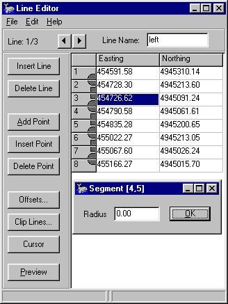
Line Editorにおいて、円弧を作成した位置は一列目の影の部分が楕円形になっているのが容易にわかると思います。
円弧形誘導測線に対してもOffsetsの操作はサポートされています。円弧形誘導測線を中心として、セクションラインを作成することができます。追加で 平行(parallel)・回転(rotated)・階段移動(shifted)の測線を作成できます。Clip Linesのオプションは円弧形誘導測線に対してはまだサポートされていません。将来的には直線の場合と同様にクリップされた円弧が作成できるようになる でしょう。
Q新しい平均断面体積計算方法(Norfolk Volume Method Added to HYPACK® MAX)[英語]
As a result of a contract with USACE-Norfolk, Coastal Oceanographics has added the ‘Norfolk’ Method as an option in the volume computation routines of the CROSS SECTIONS program. The Norfolk method is based on the average end area method of computing quantities.
It computes the entire volume above three user defined levels. In the example shown below, the design template (center channel) is at 49’. The overdepth template is at 50’, 1’ below the design. The supergrade template is placed 2’ below the overdepth template, placing it at 52’.
This routine computes and reports all of the material above the each of the three levels. The material for the side slopes and center channel is totaled to provide a total quantity available. The
quantity reported for the overdepth template contains all material above the overdepth template, including material that falls above the design template. Likewise, the quantity reported for the supergrade template contains all material above the supergrade, overdepth and design templates. This is different from the other Average End Area reports, where material is only reported up to the next template.
A sample report from the Norfolk Method is shown below.
Q曳航体の航跡処理(Towcable.dll)[英語]
During a recent training session, the towed object tracking in Hypack® was discussed with several of the Hypack® users in the class. The problem with monitoring a towed object such as a magnetometer or side scan has always been trying to approximate the actual track of the object in relation to the vessel towing the object.
After investigating the method used, a decision was made to improve the track of the towed object by using the course made good as a reference to the actual heading of the object. This worked better, but was found to be lacking a bit in the expected track of the object, so we have written a new algorithm to calculate the position.
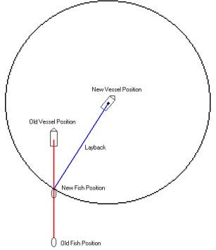
As the vessel moves ahead, a new circle is generated. The intersection of the circle and the track of the fish is then computed as the new position of the fish. The heading of the fish is the azimuth from the fish to the boat. We are still fine tuning the calculations to get a more accurate position of the fish. At this point I am much happier about the location of the towed object tracking and would recommend this method over the previous method of calculating the layback position.
If you would like the new driver I can either e-mail it to you or it can be obtained by downloading the latest Service Pack from the internet.
Below I have included a sample image of a screen capture showing both the old and new methods of tracking a towed object. This is a worst case scenario and was meant to show a dramatic effect of layback.
Q任意のエリアの体積計算(Volumes in User-Defined Areas)[英語]
In the past, we’ve had a lot of questions on how to compute volumes in user-defined polygons. If you had a Ph.D. in HYPACK®, you could usually find a way to do it, but it wasn’t easy.
With a new routine in the latest TIN MODEL program, called TrimTin, users can now ‘cut’ surface models so they conform to the edges of a user-defined polygon (border). The TIN MODEL program cuts the triangles along the polygon border and throws out the portion of the model that is outside the border. Volumes can then be computed.
For our example, I have an XYZ file of gridded multibeam data and I have a sub-area (defined by the border file) to which I want to limit the volume computation..
To create my border file, I used the HYPACK® MAX Border Editor and entered the exact XY values for each corner of the border file. I entered the last point inside the border area, to tell the TIN MODEL to keep the info inside the polygon. [I could have entered a point outside the polygon and TIN MODEL would then keep the material outside the polygon.]

The first step is to go ahead and make the TIN MODEL, using the original XYZ data file. There’s nothing new here, so I’ll skip the details. The resulting 2D model is shown in the graphic to the right.
Now it’s time to cut the tin along our border. In the File Menu, you’ll find the latest addition in an item called ‘Trim Tin’. When you click it, you’ll be asked to supply a HYPACK® MAX Border (BRD) file.
The existing TIN is now trimmed to conform to the edges of the border file. Additional XYZ data points are created at every point where a triangle leg intersects
I can now use the remaining information and run volume computations on it using any of the methods available in the TIN MODEL program. For example, the report from the Philadelphia Method is shown in the text box below.
Philadelphia Pre-Dredge Report_sample
You can see that it only provides quantities in the areas contained in the polygon and 0.0s for lines that are outside the desired area.
The same technique (TrimTin) can be used to isolate contours only in a user-desired area. In the graphic to the right, I generated contours inside the polygon area by first, making the model; second, trimming the tin to a border file; third, exporting DXF contours from the TIN MODEL on the trimmed model.
Q測地系の変換
PROJECT CONVERTERは、既存のデータを別の測地系のデータへ変換するためのプログラムです。
誤った測地系の設定で収録、編集したデータを本来の測地系のデータへ変換することが可能です。ただし、現在のところ、ローカル座標の設定には対応していません。
- 新規にプロジェクトを作成し、変換後の測地系を設定します。
- UTILITIES-GEODESY-PROJECT CONVERSIONを選択し、PROJECTCONVERTERプログラムを起動します。
- 変換対象のプロジェクトをSource Project欄より選択します。
- "1"で作成したプロジェクトをTarget Project欄より選択します。
- 変換したいファイルを選択します。
- [Add a File] :個別に変換対象のファイルを選択します。
- [Add All Files] :全てのファイルを変換対象とします。
- [Clear List].:選択済の全てのファイルを解除します。
- [Convert]ボタンをクリックして、変換を開始します。変換状況が右下のリストボックスに表示されます。
QHysweepプログラムにおける音速度補正(Sound Velocity Corrections in Hysweep Survey)[英語]
We have been getting a lot of calls lately describing multibeam data that show signs of incomplete sound velocity correction. So it seems like a good time for some notes on this topic …
Why is it important to correct for Sound Velocity?
There are two reasons. First and most obvious, in order to calculate distance with sound (which all echo sounders do), it is necessary to know the sound velocity from the surface to the bottom - the sound velocity profile.
Second and less obvious, the path of sound from transducer to bottom and back (the ray path) is not always straight. When the speed of sound varies in the water column and the beam take-off angle is not vertical, sound is refracted and follows the tortured path shown in the diagram. Fortunately, if these values (beam take-off angle and SV profile) are known, it is possible to model the ray path. This is exactly what Hysweep® does and is how it is able to give correct sounding depths for multibeam sonar.
It should be easy to see that if the sound velocity profile is measured improperly, or if the profile changes, or if the profile doesn't match the area being surveyed, multibeam depths will be wrong.
It's worth noting that the errors increase greatly as the ray paths become less vertical, which is one of the main reasons that beam angles are limited to +/- 45 degrees for Class 1 surveys.
How Often Should SV Casts be Done?
This depends entirely on the water conditions where you survey. If you survey in fresh water with lots of mixing, the Niagara river for example, one sound velocity cast per day is sufficient. If you survey in an estuary during tidal changes, it may be necessary to cast every hour or so. It is best to start out taking SV profiles frequently to understand the water conditions. Then, if only small changes are seen between casts, it may be possible to back off.
Remember that if you do not have a good SV profile there is no way to fix your data. You can however, minimize the errors due to a slightly erroneous profile by limiting the beam angles.
Entering SV Profiles into Hysweep Survey
The sound velocity profile can be entered into Hysweep® Survey either manually or through the import feature. Manual entry is just a matter of keying in the depth and velocity pairs measured by the profiler. The import method takes advantage of the fact that many sound velocity profilers create a text file which can be loaded into Hysweep® Survey. Import is better if possible because it is easy (easy is good) and less prone to errors.
To enter or import a sound velocity profile into Hysweep® Survey, use Corrections menu, Sound Velocity. The diagram shows sound velocity on the Hudson River, with a lower velocity fresh water layer resting on top of a higher velocity salt water layer.
Real-Time QC
Earlier versions of Hysweep® Survey did not make the refraction corrections for the real-time displays. The reasoning was that it is too slow to make the proper corrections and that the displays would slow way down. But we had numerous requests from customers, so we went ahead and add the refraction corrections and what a great change that was, it didn't slow down the displays as much as expected either.
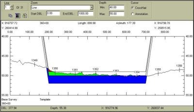
The screen shots (right) show the value of real time ray tracing for QC. The top view is corrected for refraction and the flat bottom indicates the SV profile is valid.
The bottom view is an extreme example of a bad SV profile. The edges of the sweeps are curled downward - the characteristic 'frown' of refraction errors.
Hysweep® Survey versions 0.5.21 and higher support the real-time ray tracing.