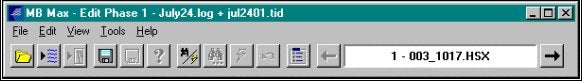
FAQ
FAQ検索結果
検索キーワード:
Qパッチテストの”不確からしさ”について(Patch Test Uncertainty)
浅海域におけるマルチビームを用いた調査ではパッチテストで安定した結果を導くことがしばしば難しいことがあります。 ロールテストでは良い結果が得られても、レイテンシー、ピッチ、ヨーではなかなか良い結果が得られないことがあります。主な原因は、DGPSのポジション精度(+/- 2 meters)のためとなっています。 ポジション精度の劣化はマルチビームのキャリブレーションやパフォーマンステストに様々な影響を与えます。今回はロール、ピッチのキャリブレーションについて説明します。
まず、ロールキャリブレーションは、なるべく平らな地形を利用して行います。これはポジションエラーによる影響を極力省くためです。真に平坦な地形を利用することは困難ですが、結果に示されるように浅海域におけるテストでも+/- 0.1 °の再現性を得ることができます。
ピッチキャリブレーションはロールキャリブレーションとは異なり少々厄介なものとなります。なぜなら浅海域におけるピッチ誤差はポジション精度に強く依存するためです。 近似式を使用するとピッチの計算は以下のようになります。
a = sin-1 ( dp / z )
a :パッチテストの結果(pitch bias angle)
dp :ポジションエラー
z :水深値
ポジションエラーとピッチバイアスの関係
|
Case |
Water Depth (feet) |
Position Error (feet) |
Pitch Bias (+/- degrees) |
|---|---|---|---|
|
1 |
300’ |
6’ |
1.1 |
|
2 |
100’ |
6’ |
3.4 |
|
3 |
40’ |
6’ |
8.6 |
|
4 |
40’ |
3’ |
4.3 |
|
5 |
40’ |
1’ |
1.4 (Very good for DGPS) |
|
6 |
20’ |
6’ |
17.4 (Yikes) |
|
7 |
20’ |
3’ |
8.6 |
Qバックホーの利用(Dredgepack on a Backhoe)[英語]
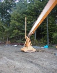
Recently an installation was performed on a backhoe running Dredgepack® with a RTK GPS. The backhoe has a rigid pole attached to the bucket. This bucket is being used to remove material from a lake. The requirements of the removal are to remove a fixed depth of material from a set area. This seems a bit confusing at first. The customer wants to remove 2 feet of material from the lake. Since most dredge operations that I have been involved in remove material to a template, this was a bit different.
To begin the project, let's start with the GPS configuration--the most important aspect of setting up the job. The customer is using an RTK system with a pre-established base station. On the backhoe, the GPS antenna is mounted to the bucket by the pole as displayed in the figure to the right. A long cable is run the length of the boom arm to the GPS receiver in the cab. The initial configuration of the RTK was very simple. Since the job site is a relatively small construction site, the datum to ellipsoid separation was entered into the antenna offsets. Once the system was communicating properly, we checked the Hypack® elevation by setting the bucket at the water surface and comparing the elevation in Hypack® with the elevation of the lake surface. The result was a perfect match! It is sure nice when the numbers work out.
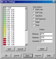
After the GPS was up and functioning, the rest of the job was simple. To show the location of the material removed we use a Matrix. The Matrix file is comprised of a rectangle divided up into cells 3 ft by 3 ft. The bucket was measured to be 3 ft by 5 ft. This was to allow us an overlap to ensure all of the material was removed. Using the Matrix in Dredgepack with the Display Difference option, the operator can then monitor the elevation of bucket and removal a set amount of depth. The Matrix colors are set to the range of material we are removing and not the value of the elevation. Our lake elevation was 108.75 ft.. Our colors were set as they are in the image to the right. The operator stops digging when the cell is Red.
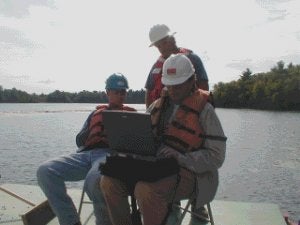
Now for the part where something went wrong. The GPS, being mounted so close to the boom, occasionally switched to RTK Float from a Fixed signal. This caused the position and depth to change drastically. After a few seconds, the Fixed RTK would be regained and the system would function properly again. The problem was that while we were updating the Matrix, the cells would fill with bad position and depth. This was due to the fact that we were not using the RTK for tide, but as an echo sounder. Had we been using it for tide, the problem could have been removed in post-processing. To find the problem required a trip to the site by Lazar. Fifteen minutes into Lazar's visit the problem was solved and we were on our way to an early lunch. ( Just kidding Pat! We were working very hard.)
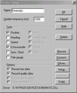
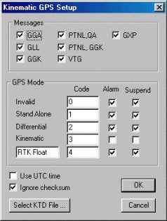
After returning to the office, a change was made to the Kinematic driver to allow the user to suspend logging where the position is less than Kinematic. The position will continue to update the data display and boat location, but no elevation or depth will be returned. This allows the user to continue to see where they are, but not to receive bad tide or depth readings that must be corrected later. This is done through the checkboxes in the GPS Mode section of the driver setup dialog. The figures below show the device setup dialog (left) and driver setup dialog (right) with the correct settings for this situation.
Q次期チャンネルデザイン(水路計画)プログラム(Advanced Channel Design 2001)[英語]
New advanced channel design program is ready for beta testing. It will replace old 16bit version but we will retain old chn data format.
I want to emphasize several new features that are implemented.
Node Editing:
- Import nodes from lnw, xyz or chn file
- Enter nodes on mouse click
- Graphic control during editing process
Face Editing:
- Graphic control during editing process
- Add toes for selected edges
- Check face integrity (flatness, orientation, convexity)
Section Editing
- Graphic control during editing process
- Multisegment sections
3D viewer:
- Interactive rotation
- 3D shading
The picture below shows screen captures of two sample channel files.
Q新しい測深データ削減プログラム(New Sounding Reduction Program for Multibeam Data)
マルチ‐ビームデータセットに関するメイン問題のうちの1つは、サーフェス・モデルを作成し、そして、巨大なデータセットからボリュームを計算することです。 このように巨大なデータを整理するためにSOUNDING REDUCTIONプログラムが用意されています。
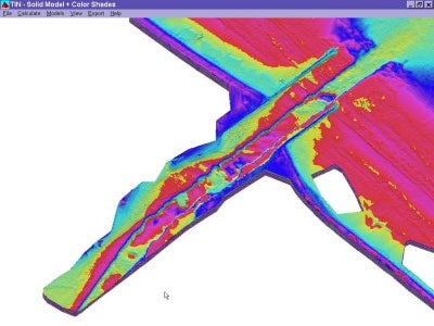
Figure 1 Original Data Set (550,499 points)
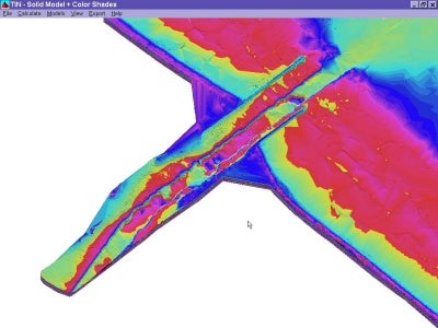
Figure 2 Reduced Data Set (60,610 points)
プログラムは、測点から構成される隣接するTINパネルの垂線ベクトルを比較します。 垂線ベクトルの交わる角度がユーザーの入力値より少ないならば、そのデータポイントを消去されます。 図2は設定値に10を入力してデータの整理をした例です。
この技術は、平滑なエリアでは効果的にデータの削減ができ、起伏にとんだエリアではその形状を正確に保つことができます。下の数字は、オリジナルのXYZデータポイント(左)を示し、そして、減少したXYZデータは、示します(右)。
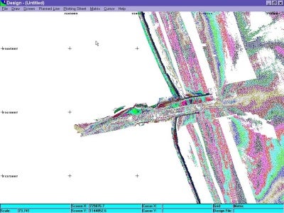
Figure 3 Original Data Set (Courtesy US LIDAR Group - Mobile, Alabama)
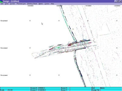
Figure 4 Reduced Data Set (10ー Reduction)
QMBMax概略(MBMax Edit Strategies)
HS2 Fileの採用
全ての編集情報が保存されるファイルが新しい編集プログラムに求められていました。そこでMB MAXではSWPファイルに替わってHS2ファイルを新たに採用しました。
複数測線データの同時読み込み:
旧プログラムでは1度に1測線分のファイルしか読み込むことができませんでした。MB Maxではコンピュータのメモリが許す限り複数の測線データを同時に読み込むことが可能です。
3つのフェーズからなる編集手順:
MB Maxは、3つの個別の編集ステージを持っています。フェーズ1は、未加工のデータ(track-lines, heave/pitch/roll, heading, tide, etc)の編集、フェーズ2は、マルチ‐ビームデータの編集。フェーズ3は、下記のFill Matrixです。
Fill Matrixの採用:
全ての水深データが表示、編集、フィルタリングのためにマトリックスファイルにロードされます。
1.データの表示。
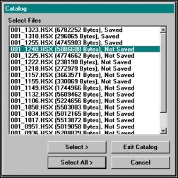
Edit-Search And FilterOptionsを使用してフィルタのセットアップをします。File-Openを選択し、データファイルをロードします。編集するデータの含まれるLOGファイルを選択し、ファイルリストが表示されたら、Select All をクリックします。
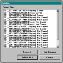
Loading Data Files
ファイルオープンオプションをセットします。Auto ProcessingオプションとApply Filtersを選択し、OKボタンをクリックします。
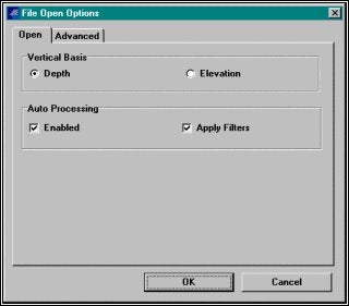
Setting File Open Options
もし既に作成されていれば補正ファイル(潮位、音速度)を選択します。
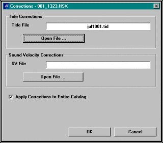
Selecting Corrections Files
マトリックスオプションの設定。オートマトリックスオプションを使用することは、最も迅速で、最も容易である。Auto‐Size to Dataは、調査範囲に適したマトリックス範囲を設定、Auto Cell Sizeは、セルの長さ、及び、幅を各セルに約50の水深データが含まれるように設定します。設定が終了したらOKボタンをクリックします。
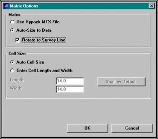
Setting the Matrix Options
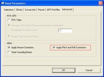
Read Parametersで適切なデバイスを選択します。OKボタンをクリックすると、MB Maxは、ファイルをロードして、フィルタ処理を行います。
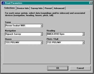
Setting the Read Parameters
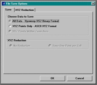
MB Maxがデータのロード、フィルタリングを終了したら、編集済みデータを保存します。File - Saveを選択します。XYZ Points Only とNo Reductionを選択し、OKボタンをクリックしてファイル名をつけて保存します。
調査データを減少させたい場合、Save One Point per Cellを選択し、XYZ Reductionタブで採用するポイント( min、max、平均等)を選択します。
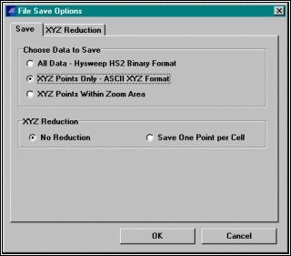
Saving your Edited Data
Hypackで調査データを表示する場合、File - Save Matrixを選択し、名前を付けて保存します。
2.変更
MB Maxは、旧スィープエディタとほとんど同じ様に使用できます。ファイルをロードし、それを編集、そしてセーブする、別のファイルをロードする、それを編集し、それ等をセーブする。異なる点は個々のファイルをSWPフォーマットに保存しない点です。データファイルを選択します。File – Openを選択し、LOGファイルを選択します。ファイルリストが表示されたら、Select >ボタンをクリックして、編集するファイルを選択します。
Loading your Data Files
オープンオプションでAuto Processingを無効にします。
補正ファイル(潮位、及び、音速度)を選択します。
Read Parametersで適切なデバイスを選択します。
編集段階1 :ファイルが読み込まれるとrawデータウィンドウが表示されます。
Tip: ウィンドウを容易にアレンジするために、View - Tile Windows (或いは、Ctrl-F9 )を選択します。すべて終了したらFile - Convert Raw to Correctedを選択しフェーズ2に移行します。
編集段階2 :編集、及び、フィルタリングは、旧スィープエディタとほとんど変わりません。編集が終了したら、編集されたデータを保存します。File – Saveを選択します。File Save OptionsでAll Data - Hysweep HS2 Binary Formatを選択し、OKボタンをクリックします。ファイルは、拡張子hs2で未編集のファイルと同じ名前でエディトフォルダーに保存されます。
Saving the Edited Data
次のデータファイルをロードし、このプロセスを繰り返します。
個々のデータを編集し、保存した後、編集されたデータの全てをXYZフォーマットで保存してください。
再びFile – Openを選択し、カタログを出ます。
エディトフォルダーからカタログを選択しSelect Allで全てのデータを選択します。
ファイルがロードされたらF4を押下し、変換を実行します。変換終了後、File - Saveを選択します。今度はHS2フォーマットではなくXYZフォーマットを選択します。ここで作成されるXYZファイルは、全ての編集された水深値を含み、ExportやHypack Mapperプログラムで使用することが可能です。
Note :これらの処理では、編集段階3を使用していないことに注目してください。
3.基本
この過程の大部分は、コンピュータによって処理されます。
データファイルをロードします。File - Openを選択し、LOGファイルを選択します。ファイルリストが表示されたら、Select All >をクリックします。
オープンオプションでAuto Processingを無効にします。
補正ファイル(潮位、及び、音速度)を選択します。
Read Parametersで適切なデバイスを選択し、OKボタンをクリックします。
編集段階1
:rawデータグラフが表示されたら、ウィンドウをアレンジするためにCtrl-F9を実行します。
不安定なヒーブデータの確認
不安定なヒーブとは下図のような状態です。
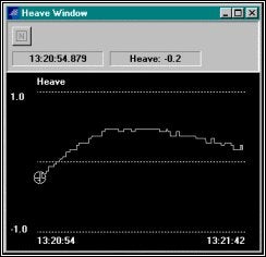
Unsettled Heave
これは船が急旋回し、補正装置が安定する前にデータ収録を開始したことが原因でしょう。このことは他の何より浅海でのマルチビーム調査を質の悪いものにします。それを修正するために、マウス(この場合、隆起全てが悪い)で悪い隆起部分をブロックし、Fill Blockツール(左上)をクリックしなさい。全ての隆起値を満たすため、0を入力し、OKボタンをクリックします。
GPSエラーデータの確認
GPSポジションスパイクは、下のSurveyウィンドウにおいて示されます。1つのポイントを取り除くためには、それをクリックし、そして、Deleteキーを押下します。ポイントをまとめてを削除するためには、Block Toolをクリックし、マウスでスクリーンに選択範囲を描画します。その後、Delete Inside、または、Delete Outsideボタンをクリックすることでエラーポイントの削除が実行できます。
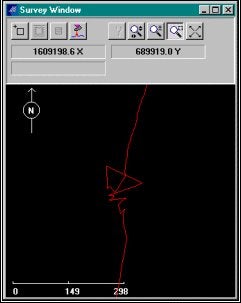
Position Spikes in the Survey Window
他のセンサーについても確認
残りのセンサをチェックするのは、グラフからそれらが正しい(データスパイク、完全にフラットな部分など)動作をしていたか確認します。
次の測線データに移動するにはMB Maxタイトルウィンドウの右矢印ボタンをクリックします。
Changing Data lines in the Multibeam Max
データの全てをセーブするにはFile - Saveを選択し、オプションでAll Data - HS2 Binary Format 選択後、OKボタンをクリックします。編集フェーズ2に移行するためにF4を押下します。
編集段階2
オートフィルタによって全ての明らかに悪い水深データを取り除いてスタートします。Edit - Search and Filter Optionsを選択します。
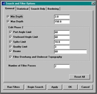
Setting Search and Filter Options
Minimumとmaximum depthは、特別な意味はありません。
Port and starboard angle limitsは、調査タイプ(浚渫、コンディション等)に応じて通常定められます。
spike filter限界が適度に大きい(水の深さの10%を言う)とき、スパイクフィルタは、安全です。しかし、沈船や障害物の調査をしている場合は使用しないでください。
quality filterは、マルチ‐ビームソーナからのコードに基づいており、そして、悪いと知られているあらゆるビームがあるならば、それらを除去します。
Filter overhang、ウォーターカラムにおけるノイズを真の特徴を取り除かないで除去するのに役立ちます。フィルタのセットアップが終了したら設定が有効になるようにRun Filtersボタンをクリックします。
フィルタを実行した後で最初のラインをスクロールし、そして、水深データを検査します。残っているエラーデータを1ポイント、 または、ブロック単位で削除します。編集フェーズ2においてポイントを削除するためのアドバイスは「疑わしい場合は残す」です。カタログを終えるまで、各ラインのプロセスを繰り返します。
再び全てのファイルをHS2フォーマットでセーブします。
この点で、あなたは、適度にクリーンなデータセットを持っているべきです。それは、今残された問題の水深測量の更なる検査に関わる問題の解決は編集フェーズ3で行われます。
編集段階3:File - Fill Matrixを選択します。このフェーズにおいて、マトリックスは、水深データをまとめ、統計の比較、及び、表示のためにために使われる。しかし、Mapperプログラムと異なり、全ての水深データは、保持されます。
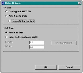
Setting Matrix Options for Gridding your Data.
Auto Size to Dataは、調査範囲に適したマトリックス範囲を設定、Auto Cell Sizeは、セルの長さ、及び、幅を各セルに約50の水深データが含まれるように設定します。設定が終了したらOKボタンをクリックします。
編集段階3 :全ての水深データをマトリックス構造化するのは、別の長いプロセスで行います。マトリックスが満たされるとデータの3つのビューが利用可能になります。
Survey ウィンドウ: 塗りつぶされたマトリックス
Profile ウィンドウ: マトリックスの行または列方向によって切られた断面
Cell ウィンドウ: 現在のセルにおける全ての水深データ
統計のSearch and Filter Optionsセットします。Edit - Search and Filter Options選択します。それぞれのセルの参照となる深さとして使用される統計を選択します。また、参照点から上限または下限の受入れ限界を設定しま す。多くの場合Medianは最適なセッティングとなります。Limit値は1 ~ 3フィートが最適値です。やわらかい底質では1フィート、岩盤では3フィートが最適でしょう。
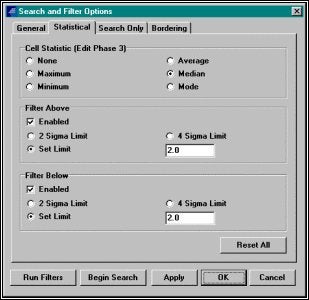
Setting Statistical Filters
statistical filtersが設定されたら、Begin Searchボタンをクリックします。MB Maxは、検索条件を越えるセルのデータをスキャンし始めます。条件を超えた水深データが存在しているとき、MB Maxは、それを含むセルを表示します。Survey ウィンドウにおいて、そのセルは、照準用十字線によって表示されます。Profile ウィンドウでは、垂直のバーによって表示されます。Cell ウィンドウでは、黄色のXマークによるセルの中の全ての水深データがフィルタ限界の外のものであることを示します。
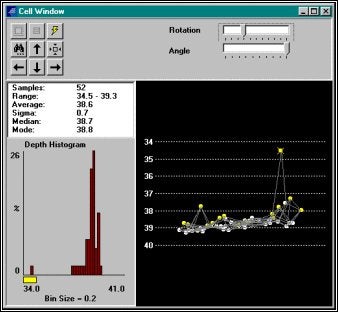
Viewing Soundings in a Cell Where Some are Outside the Filter Limits
ここでこの測深データが良いのか悪いのか決定しなければなりません。:この水深データは、この場合悪いように思われるでしょう。残りのデータよりかなり上にあります。しかし、それを除去する前に、周囲のセルの水深データを見るために、Include Neighboring Cellsツールをクリックします。すると、それが分離したポイントではないということ、そして、その特徴が1を超える調査ラインによるものだということが明確に解ります。
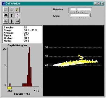
Viewing the Same Data with Data from the Surrounding Cells
どのようなデータを削除すれば良いか?
オーバーラップすることのあるエリアにおいて、片方のみに存在するデータを取り除くことは、安全です。だが注意する必要があります。水平の正確度の問題により、該当データは、異なるラインの異なるロケーションに存在するかもしれません。
いくらかの機関、及び、契約者は、水深測量を受け入れるために彼ら自身の規則を設定しています。例えば、2個以下であれば除去し、3個以上であれば保持などです。
それ以上は個人判断に関わる問題でしょう。セルウィンドウにおける回転、及び、角度スライダは、様々な角度からの確認を用意にしているので活用してください。
データの削除:
全てのXマーク水深データ( Cell ウィンドウのみで)を取り除くためにはCell ウィンドウでFilterボタンをクリックします。
Deleteキーで1つ1つ削除削除するかブロック単位で削除します。次のポイントを検索するためにはFind Nextボタン、または、F3を使用します。
Profile ウィンドウは、検索プロセスにおいて役立ちます。垂直のバーは、現在のセルのポジションを示します。例は、オーバラップが容易に比較できるようにライン番号によるカラーコーディングがされています。
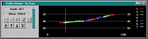
Viewing Data in the Profile Window
全てのセルが検索された後で、シンプルな結果が表示されます。
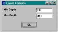
Post-editing Summary
最後にHS2 (再編集が必要とされる場合)と、XYZフォーマット(更なる処理のために)の両方でデータを保存します。
QローカルグリッドにおけるGPS使用の注意(Working on a Local Grid Using GPS)
時折、多くの測量士が、ローカルグリッド上で調査を行う必要があります。これらのローカルなグリッドは、各現場の要求に合うように起点、回転角が設定されます。それに加えポジショニングには使用しやすさとその精度からGPS を使用します。ここで問題となるのはGPSの出力するデータはローカルグリッドではなくWGS-84に基づいているということです。そこで、測量士は、そ のWGS-84の緯度・経度をローカルなグリッド座標に変換する作業が必要となります。この変換作業はHYPACK MAX可能です!
この変換を行うために、調査エリアに少なくとも2つのテストポイントが必要となります。あなたは、それらのポイントのローカルな座標、及び、投影における同じポイントのための座標値を知っている必要があります。
HYPACK、®MAXのGEODETIC PARAMETERSプログラムで利用可能な投影は平面座標系、及び、UTMシステムのうちのどちらかです。
以下、下記に揚げる例を使用して説明します。:
| Point # | ローカル座標 | NAD-27 北フロリダ座標 |
|---|---|---|
| 1 | X = 4000.00 Y = 25000.00 |
X = 2779078.11 Y = 368284.56 |
| 2 | X = 4500.00 Y = 25000.00 |
X = 2779577.98 Y = 368296.18 |
| 3 | X = 4500.52 Y = 30346.25 |
X = 2779454.27 Y = 373641.14 |
| 4 | X = 4240.35 Y = 30641.85 |
X = 2779187.30 Y = 373930.62 |
異なるセットポイントの間の相対距離、及び、回転角を比較するために、私は、ローカル座標系とNAD-27座標系グリッド北からの方位差を計算します。北方 向の座標差を東方向の座標差で除算した値のアークタンジェントとることによって算出されます。(ただし、どのような象限にいるかに対する注意を払う必要が あります。)
| Point Pairs | ローカル座標上の方位角 | 平面座標上の方位角 | 差 |
|---|---|---|---|
| 1-2 | 90.0000 | 88.6683 | 1.3317 |
| 1-3 | 5.3485 | 4.0169 | 1.3316 |
| 1-4 | 2.4394 | 1.1079 | 1.3315 |
| 2-3 | 0.0056 | 358.6741 | 1.3315 |
| 2-4 | 357.3650 | 356.0336 | 1.3314 |
| 3-4 | 318.6476 | 317.3165 | 1.3311 |
|
Average |
1.3315 = 1º 19' 53.4" |
| Point Pairs | ローカル座標上の距離 | 平面距離 | 縮尺率 |
|---|---|---|---|
| 1-2 | 500.00 | 500.005 | .999990 |
| 1-3 | 5369.628 | 5369.772 | .999973 |
| 1-4 | 5646.967 | 5647.116 | .999974 |
| 2-3 | 5346.250 | 5346.392 | .999973 |
| 2-4 | 5647.822 | 5647.968 | .999974 |
| 3-4 | 393.786 | 393.791 | .999987 |
|
Average (long distances) |
.999974 |
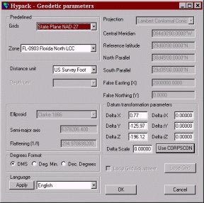
最初にGEODETIC PARAMETERS でNAD-27フロリダ北方平面座標系のセットアップを行います。Grids欄をState Plane NAD-27’にセットし、ZoneにFL-0903 Florida North LCCにセットします。この場合、楕円体はWGS-84 、GRS-1980のいずれでもないので、データ変化をしなければなりません。
Use CORPSCONボタンをクリックし、そして、適切な緯度‐経度を入力します。
本例の場合は下記の緯度経度を入力します。
緯度= N29º59’ 23.42416
経度= W82º02’ 19.37624
CORPSCONデータベースから抽出されたパラメータは以下の通りです。
デルタX = 0.77
デルタY = -125.97
デルタZ = -196.12
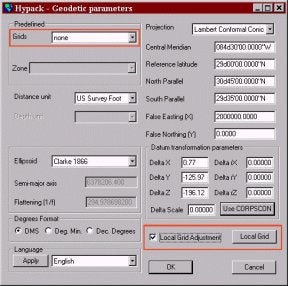
Local Grid Adjustmentパラメータを設定するために、Grid欄にnoneを設定します。その後、Local Grid Adjustmentをチェックすると、Local Gridボタンをクリックすることが可能になります。
[Grids欄に‘none’にセットしない限り、このエリアにアクセスすることができません。]
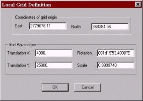
計算された情報に基づいて、次のパラメータを入力します。:
Coordinates of grid origin 欄にポイント1のフロリダ北方平面座標系の座標値を入力します。
Grid Parameters欄にポイント1のローカル座標及び、前のページで計算されたRotation、Scaleを入力します。
Local Grid Definitionウィンドウを閉じ、GEODETIC PARAMETERSを閉じます。
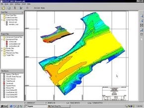
これをテストする最も良い方法は、Utilities – GeodesyのGRID CONVERSIONプログラムを使用することです。このプログラムは、WGS-84系の緯度経度をローカル座標系の緯度経度に変換し、そして、それを平面座標系に変換します。
Qパッチテストの”不確からしさ”について(Patch Test Uncertainty II)
レイテンシーテストのための測線ラインは、同じ方向を様々なスピードで海底地形を測量することによって行います。2つのオーバーラップしているラインが必要になります。全てのパッチテストと同様に、結果は、位置決めの精度によって変わります。同じくレイテンシーの結果は、異なるボートスピードによって変わります。それは、水深さによって変わることはありません。
レイテンシーをポジションエラー、及び、スピード変更と関係づける方程式は、簡単ではありません。:
レイテンシー= dp / ds
ここで、
latency:パッチテストの結果(GPS latency),
dp:ポジションエラー,
ds:船速の変化(ノット) ,
| Case | Position Error (feet) | Differential Speed (knots) | Latency Bias (seconds) |
|---|---|---|---|
| 1 | 1 | 2 | 0.29 |
| 2 | 1 | 4 | 0.15 |
| 3 | 1 | 8 | 0.07 (very good) |
| 4 | 3 | 2 | 0.88 |
| 5 | 3 | 4 | 0.44 (典型的な値l) |
| 6 | 3 | 8 | 0.22 |
| 7 | 6 | 2 | 1.76 |
| 8 | 6 | 4 | 0.88 |
| 9 | 6 | 8 | 0.44 |
最も良い結果は、最も小さいポジションエラー( duh )と最も大きい異なるボートスピードで得られます。典型的なコンディションの場合、レイテンシーテストの結果は、約0.5秒で異なります。それは、現実の 待ち時間より多いかもしれません。よりよい結果を得るためには、履歴をたどり、エラーを取り除くために多くのテストに関する平均結果を使用してください。
船速に関する考察:
スピード差を増加することが、更に良い結果を提供することを理解することは、容易です。より低いスピードで、測線に留まることは、難しいかもしれません。 また、より高いスピードでは、音響品質は、悪化するかもしれません。マルチビームを使用する多くの測量士は、より良い結果を得るために試行錯誤を行いま す。スクワット変異を追跡し、垂直オフセットを適応することも同じく重要です。
また、マルチビームオフセットとしてレイテンシーを入力してはいけません。それは、GPSのオフセットです。
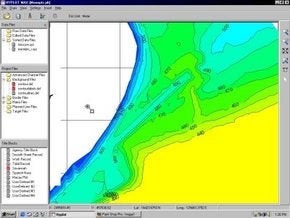
Q新しいHyplotプログラム(New Hyplot Program)
HYPACK MAXでは近い将来HYPLOT MAXと呼ばれる新しいプロットプログラムが採用されます。
HYPLOT MAXの主な特徴は下記のとおりです。:
- Windows® プリンタドライバを使用したプロッタ、プリンタ出力
- ネットワークを使用したプリンタ、プロット出力のサポート
- BMPとJPGグラフィックファイルのサポート
- 出力イメージの拡大、縮小、パンが可能
QDXFファイルを測線ファイル(*.lnw)へ変換(Reformatting DXF files to Planned Line Files in Reformat)
ユーザーは、DXFファイルをHYPACK(TM) Planned Line(計画測線) ( *.lnw )ファイルに変換することができます。AutoCAD、または、他のCADパッケージにおいてあなたの計画測線を設計し、そして、これらをLNWファイルとして使用することができます。
作成されたDXFファイルをただしくLNWファイルに変換するために、さ区政された測線は、 PLANNEDLINESと指定されたレイヤーに位置している必要があります。このレイヤーには変換しないオブジェクトは載せないようにしてください。図 1は、AutoCADで作成した水路と測線を示しています。
Figure 1: AutoCAD dxf drawing
HYPACKのメインウィンドウで、Final Products – Exportを選択します。いったん、そのプログラムがアップし、そして、起動した画面のConvert Fromリストから*.DXFを選択します。一度DXFファイルを選択すると次からSelected Filesリストに自動的に表示されるようになります。File – Convertを選択すると変換後の測線ファイル名を指定するように促されます。Saveボタンをクリックすると変換が実行されます。
Figure 2: HYPACK(TM)’s Reformat program
これらのラインファイルはテンプレート情報を全く持っていないので、個々のテンプレートを作成せずに体積計算をすることはできません。
Figure 3: LNW file created in Reformat program
Qサーベイノート(Survey Notes in MAX)[英語]
This note is regarding the Target Editor as well as notes recorded by Survey. The problem arose when a survey crew spent a full day collecting targets. At the end of the day it was realized that there was a target that needed to be added to the list. The surveyor took the target file and opened it in the Target Editor program. He then elected to insert a target to the beginning of the file. This caused a line to be inserted at the beginning of the target list. The next step is where the problem came in. He chose to add the point with the cursor. This caused the program to clear the list of targets previously held in the file and start a new list. Once he was done adding targets the surveyor saved the file. He did not notice that the targets had been removed.
Now that we have found that the targets have been removed we can figure out a way to recover a days worth of work. This is the Survey Notes I referred to earlier. A short time ago one of our programmers wrote a function into the Survey program. This function writes a text file for every day that you run the Survey program. I am going to include a sample to show what is recorded.
The following is an example with a short description of each item.
<10:42:59> PROJECT NAME: Ross_Island
<10:42:59> PROJECT DIR: C:\HYPACK\Projects\Ross_Island\
>> Header to let you know what project this file is from.
<10:42:59> Using Line 1 from C:\HYPACK\PROJECTS\ROSS_ISLAND\
LINE1.LNW
>> Lists the current line file in use.
<10:42:59> No Matrix File selected
>>Lists the Matrix file Selected
<10:42:59> Opening Data File C:\HYPACK\Projects\Ross_Island\
RAW\001_1042.RAW
>> What time was the line started to be recorded.
<10:42:59> Event #1
>>Event #1 occurred
<10:42:59> NMEA Warning: No Sync
>> The Position was set to Sync Clock and it failed.
<10:43:00> XTE Limit = 20, XTE = -2247890
>> The cross track limit was exceeded
<10:43:15> Closing Data File C:\HYPACK\Projects\Ross_Island\
RAW\001_1042.RAW
>> Closing the data file
Later that day the Survey was continued and the following is also a section recorded in the same file. Everything that happens in Survey is written to a single file for each day. This section is appended to the file with an empty line separating the data segments. The important part of this file is that we recorded a group of targets. You can see that the time and X,Y of each target is recorded in the file. Luckily the surveyor from my example was able to recover the targets by using this file. There is no substitute for taking good notes and this is a prime example of it. We took notes without even knowing how important it would become.
<14:25:07> PROJECT NAME: Ross_Island
<14:25:07> PROJECT DIR: C:\HYPACK\Projects\Ross_Island\
<14:25:07> No Line File selected
<14:25:07> No Matrix File selected
<14:25:07> Opening Data File C:\HYPACK\Projects\Ross_Island\
RAW\000_1425.RAW
<14:25:07> Event #3
<14:25:07> NMEA Warning: No Sync
<14:25:08> Event #4
<14:25:08> Closing Data File C:\HYPACK\Projects\Ross_Island\
RAW\000_1425.RAW

<15:00:25> Target 15:00:25 (1016871.17, 740807.55)
<15:00:25> Target 15:00:25 (1016871.17, 740807.55)
<15:00:26> Target 15:00:26 (1016871.17, 740807.55)
<15:00:26> Target 15:00:26 (1016871.17, 740807.55)
<15:00:26> Target 15:00:26 (1016871.17, 740807.55)
<15:00:26> Target 15:00:26 (1016871.17, 740807.55)
<15:00:27> Target 15:00:27 (1016871.17, 740807.55)
Q曳航体の動きについての考え方(Towed Object Layback Method in Hypack® Max)[英語]
During a recent training session, the towed object tracking in Hypack® was discussed with several of the Hypack® users in the class. The problem with monitoring a towed object such as a magnetometer or side scan has always been trying to approximate the actual track of the object in relation to the vessel towing the object.
After investigating the method used, a decision was made to improve the track of the towed object by using the course made good as a reference to the actual heading of the object. This worked better, but was found to be lacking a bit in the expected track of the object, so we have written a new algorithm to calculate the position.
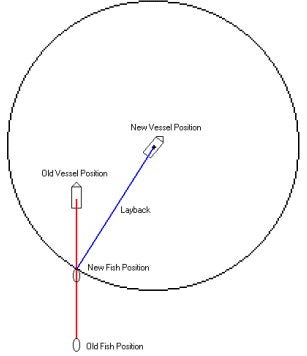
As the vessel moves ahead, a new circle is generated. The intersection of the circle and the track of the fish is then computed as the new position of the fish. The heading of the fish is the azimuth from the fish to the boat. We are still fine tuning the calculations to get a more accurate position of the fish. At this point I am much happier about the location of the towed object tracking and would recommend this method over the previous method of calculating the layback position.
If you would like the new driver I can either e-mail it to you or it can be obtained by downloading the latest Service Pack from the internet.
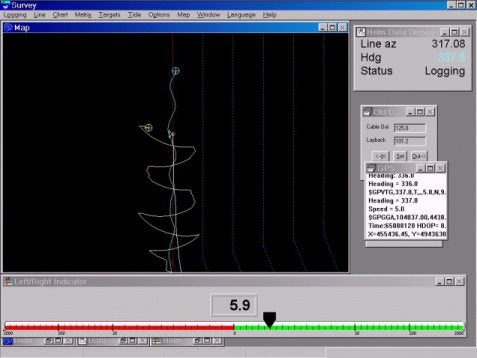
Below I have included a sample image of a screen capture showing both the old and new methods of tracking a towed object. This is a worst case scenario and was meant to show a dramatic effect of layback.
Qマトリックス表示オプション(Display Options for Matrix Files Used in Dredging)[英語]
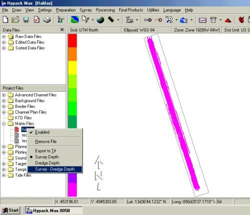
Most users view Matrix files as two dimensional objects, that is as a (row x col) grid. A third dimension, the Depth, is contained inside each cell of the matrix. The matrix structure also has the capability of storing an additional depth for each cell, which gives a stacking of depths projecting from the surface of the screen. This feature is used in Dredgepack® for recording the pre- and post-dredging depths of a given area. You can display the Survey Depth, the Dredge Depth or the Difference between the two depths (Survey-Dredge Depth) in Dredgepack® by selecting it through the Matrix menu.
There is a new option in HYPACK® Max that supports this display in the main Max window. Users with a Dredgepack® or Universal key can select which depth to view by right clicking on Matrix Files in the Project Files list and selecting the appropriate option from the menu. If the cell is missing either the Survey or Dredge depth, then the cell will display blank in the difference mode. The screen capture below gives an idea of how it works.
Qシングルビームにおけるロール、ピッチ補正について(Pitch and Roll Corrections in Sbmax)[英語]
When a single beam survey is done in calm water conditions, there isn’t much need to measure the pitch and roll of the boat. Because there is none. But as water conditions become rougher, sounding errors due to boat motion begin to increase and pitch and roll measurements can significantly reduce those errors.
In HYPACK®, pitch and roll compensation is done in the editing stage of post-processing – the Sbmax edit program. A number of people have asked: how exactly does Sbmax correct for roll and pitch. Hmm, sounds like a good topic for Sounding Better…
We consider the simple case of the GPS antenna mounted directly above the transducer. When there is no pitch or roll, the horizontal position of the antenna is exactly the same as the transducer and there is no sounding error.
When the boat rolls, the antenna is going to move one horizontal direction and the transducer is going to move the opposite direction – the pivot point of rotation being directly above the keel at the waterline. Without compensation, this will lead to a position error. Additionally, roll will cause the transducer to move slightly upward, changing it’s draft and causing a slight depth error.
The little stick diagram illustrates the roll rotation and it’s effect on the position of the transducer relative to the GPS antenna. Although not shown, pitch rotation will have a similar effect, with the pivot in this case at the boat center of mass.
Sbmax pitch and roll compensation uses standard mathematical formulas to correctly transform the transducer position relative to the antenna. The end result is that the transducer position is corrected to give the correct sounding position and the transducer draft change is compensated giving the correct depth. Note that in order for this to all work properly, the Hypack boat origin should be specified at the boat center of mass (approximately).
Pitch and roll corrections are enabled with the check box in Sbmax Advanced Read Parameters: Apply Pitch and Roll Corrections.
If you are interested in what happens when you check “Steer Sounding Beam”, refer to Sounding Better, February 2001: Beam Steering in the Single Beam Editor.
QXYZ入力プログラム(XYZ Collector)
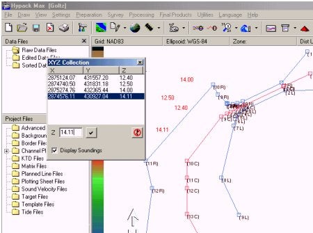
処理の途中でXYZファイルを作成する新たな機能が追加されました。新しいXYZ CollectorはHYPACKMAXのメインメニューまたは、ツールバーのショーカットから起動します。エディターが開いたら、座標値を入力したいポ イントをマップ画面上でダブルクリックします。エディター上にダブルクリックした位置の座標値が表示されたら、エディター下部のZ入力欄に水深を入力後 チェックマークのついたボタンをクリックします。
作成したXYZファイルは、現在のプロシェクト内の\Sort\sounding.xyzとして保存されます。このファイルはEditorを起動、終了するたびにアップロードされます。
簡単な例を以下図に示します。
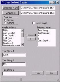
Qユーザー定義のデータ出力(User-Defined Output)
User-Defined Outputは、最新のHYPACKR Maxで追加された新しいユーティリティープログラムです。このプログラムは、編集済ファイル(ALL Format)を分解し、そのファイルに含まれる 情報をユーザが指定したファイルに書き出す事が可能です。このプログラムは、ログ ファイルや個々のデータファイルを入力として指定できます。同じような 機能を持つExport (Reformat) プログラムは多くの出力オプションを持っていますが、私たちは多くのユーザーから標準的なXYZファイルの様々なフォーマットの出力要求を受けてきまし た。(例:event XYZ, XYZ Tide, YXZ等.)。そこで、 Export プログラムにこれらのフォーマットを追加するよりはむしろ、ユーザが定義した様々なフォーマットに対応した出力ができるツールのほうが役立つだろうと考 え、User-Defined Output プログラムを用意しました。
操作手順を以下に示します。
プログラムを実行し、抽出元となる編集済ログファイル等を選択します。さらに、出力するファイルの名前も決定します。"Available" 項目のリストを参照して出力したい項目を選択します。"Available"項目のリストには3つのユーザ定義文字列も含まれます。項目を選択した後、選 択した項目の順序でファイルに書き出されます。また、各項目をコンマやスペースを使って区切る事や水深値の符号を逆にする事も可能です。
User Defined Output Program
Output file created from User Defined Output Program
QDesignプログラムで作成した測線(LNW)をSurveyプログラム上で読み込んでいるのですが現在の船の位置よりかなり離れた場所に表示されます。何が間違っているのでしょうか?(下図参照)
- 測線(LNW)を作成する時のXY座標の入力は合っていますか?
HYPACKでは、南北が"Y"、東西が"X"の数学座標を使用しています。(下図参照)
- 測線(LNW)を作成した時の測地の設定(Geodetic Parameter)とSurveyで使用している測地の設定は一致していますか?もし異なっているようであれば、正しい測地系の設定に変更してください。
Q5:SurveyプログラムのWindowメニューでTSSのデータを確認すると正しく来ているのに画面下に"Heave"と赤く表示されるのはなぜでしょう?
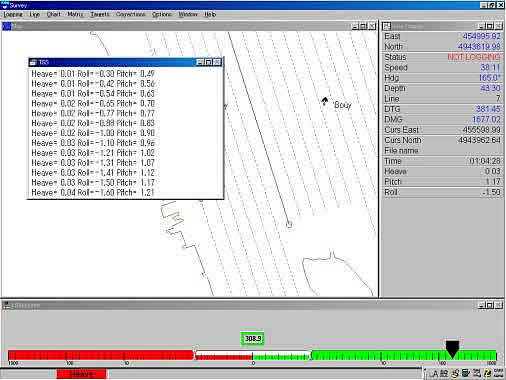
A5:HYPACKを終了し、DMSView又はターミナルソフトを使用してTSSからのデータ見て下さい。
データ中に含まれているフラグが小文字になっていませんか?(下図参照)
これは、何らかの原因でセルフテスト実行中である事が考えられるので大文字の"U"になった後に測量(Survey)を開始して下さい。
023DE7-0007u 00230038
023DF6-0007u 00160041
053E1C-0007u 00090044
QWindows2000,Xp上でのHypack8.9の動作について
HYPACK 8.9はWindows 3.1にも対応した豊富なコードを持つアプリケーションです。これは16Bitで書かれたプログラム及びデバイスドライバだと言うことです。Window 2000はWindows NT 4.0と同じく32Bitで動くOSです。HYPACK 8.9のコードがWindows 2000上でどのように取り扱われるかが問題となってきます。
我々がWindows 2000にHYPACK 8.9をインストールしたときは、正しくインストールされ、Hardlock Device Driverを使用することもできました。このプログラムはHardlock Keyの製作者よりWindows 2000がリリースされる前に供給されたものです。この会社はWindows 2000がリリースされた後に新しいバージョンのデバイスドライバを作成しました。このプログラムはHYPACK MAXに標準的に使用しているバージョンです。このプログラムはHardlockとラベルされたHYAPCK CDのサブディレクトリにあります。もしPCにHYPACK 8.9しかインストールされていない場合は、HardlockデイレクトをCoastalディレクトリの下に上書きコピーしてください。郵送されるHYPACK 8.9はWindows 2000には対応していません。新しいHardlockプログラムを入手したい場合は、お問い合わせ下さい。
HP Pavilion 6545:Celeron 500 MHzでテストを行いました。別のPCを用意し、そこからNMEA GGAを出力させ、Windows 2000PCでHypack 8.9のSurveyを実行しましたが特に問題は見られませんでした。
HardwareとSurveyプログラムでテストした後、Single Beam Editorでのテストを行いましたがこれも問題ありませんでした。その後、CoastalディレクトリにあるDam7000.xyzを用いTIN Modelプログラムを走らせました。この結果、非常に速い処理を経た後、問題無くTinデータを生成することが出来ました。
結果として、Windows 2000でHypack 8.9を走らせても問題ないと考えられます。ただし、これは全く問題がないというわけではありません。まだ、発見されていない問題が隠れているかもしれま せん。新しいバージョンのWindowsを使用する際は最新のHypack Maxを使用してください。
Qクロスセクション(断面と平均断面計算)プログラムにおけるテンプレートの使用(Custom Templates in Cross Sections and Volumes)
最近、色々な形状の水路をメンテナンスする顧客が出てまいりました。(下図参照)
彼らは、HYPACK MAXで水路の型と計画測線を自動で作成してくれるCHANNEL DESIGNを利用します。CHANNEL DESIGNは水路の深度とサイドスロープの情報に沿って、左トーライン・センターライン・右トーラインの情報を入力するだけでLNWファイルが自動的に作成することができます。
測量し編集されたデータをCROSS SECTIONSプログラム実行時に水路の体積計算を行うために読み込みます。断面図の例を下に示します。取り除くべき土の総量は320000yd3以上でこのプロジェクトでの量を超えています。
取り除くべき土の総量を減らすため、この機関では注目するエリアを縮小することにしました。彼らは取り除くべき部分のラインを左トーラインより30m内側に変更しました。つまり水路のセンターライン沿いに似たラインを作ることにしました。(下図参照)
この情報はプロットされ、元のラインから両岸の人工エリアまでの距離が測られました。
元のデータファイルをCROSS SECTIONプログラムでロードします。Template Editorを使い、新しい水路断面の形情報を入力しセーブします。この手順を各測線で繰り返します。
下図の例では、4 点のテンプレートがあります。最初の点は中心線の表面(深度0)から191.7mの位置にあります。2番目の点はそこからまっすぐ下29mで、新しい水路 の左端は井戸のように垂直になっています。3番目の点は中心線から341mで深さは29m、4番目の点はそこからまっすぐ上で、341mの位置です。
このテンプレートと水路断面は下図のように表されます。(CROSS SECSIONS – Viewerより) 両端が垂直の井戸のようになっているため、V1L、V2L、V1R、V2Rの量はありません。全体の土の量はV1とV2です。
この手順を全測線に対して繰り返します。単純な作業でこの例では30分くらいかかるでしょう。
もし水路が同じ断面をしているようならば、1つのテンプレートだけで水路全体をカバーできるでしょう。
全部のテンプレートができあがったら、全土量を確認します。下図のように示されます。
Qデータ変換プログラムの7つのパラメータ(New 7-Parameter Datum Transformations Program)[英語]
Mircea Neacsu has recently completed a new program that allows users to calculate the 3-parameter or 7-parameter datum transformation parameters from a list of geographic coordinates.
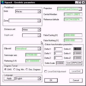
For our example, I want to compute both the 3-parameter and 7-parameter transformations for the island of Macau. Macau operates on an Azimuthal Equidistant projection that is based off the International ellipsoid.
To get started, I have made a HYPACK MAX project and called it Macau. I have set the geodetic parameters to the local Macau grid, as it is a pre-defined grid available from the menu. What is missing is the Datum Transformation information.
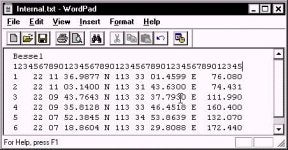
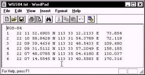
I have a list of six points on the island. One list is in WGS-84 and the other list is in International. I have typed the two lists into a TXT file (using Notepad), using a fixed format so that all the items are aligned. This will be important later on. I also have a typo in the Internal.txt file. I entered "Bessel" as the first word. This doesn't matter, as the program is going to read the GEODETIC PARAMETERS from the project and figure out that it is really an International ellipsoid.
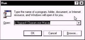
I then start the program from the Run menu. Since this is so new, there is not yet a MAX menu item for the program. The program is in the \HYPACK directory. You need to add a space after the name of the program and then enter the name of the project. The program will read the geodesy from the named project to figure out what ellipsoid you are working on.
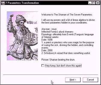
When the program first starts, it puts up this humorous screen, providing a few details and insights. After you get tired of reading it, you can click the "Very funny…" box and you won't have to read it again.
Click the "Next" button and you are taken to the next window.
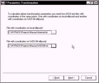
In this window, I give it the name of the two TXT files that have the geographic coordinates (Lat, Long and Ellipsoid Height) for each of the data points. These files can be anywhere on your computer or network.
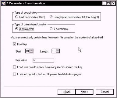
In the next window, I start by telling the program that my TXT files contain "Geographic coordinates".
I can then select to determine the best 3 parameter or 7 parameter transformation that fits the data points.
The "Use Key" option allows you to ignore any line in your text file that does not contain the "Key" letter. In our case, we are looking for the letter "N" in the 19th column of each line to denote a record we want to use.
The "Load files now to check how many records match the key" will pre-read each of the files and show you how many points have met the "key" criteria. You want the same number of points in each file.
The "I defined my fields before. Skip over field definition pages" will proceed directly to the computation. If you haven't defined your fields (and I haven't defined them yet), don't check this. Once you have defined where the information in your TXT files is placed, you won't have to go through this every time.
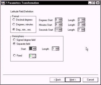
In the figure to the right, I have defined where to look in each record for the latitude information.
I am reading Degrees-Minutes-Seconds from each record. The degrees start in column five and are two characters long. The minutes start in column 8 and are two
characters long. The seconds start in column 11 and are 7 characters long.
My hemisphere identifier (N) is in column 19.
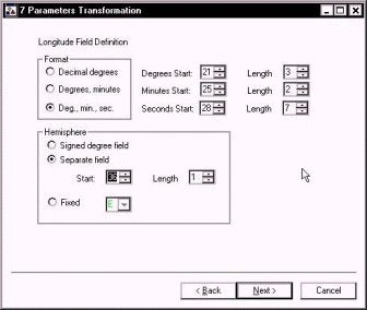
In the next window, I do the same for my longitude information.
The format is once again Degrees-Minutes-Seconds.
My degree information starts in column 21 and is 3 characters long. My minute information starts in column 25 and is two characters long. My seconds value starts in column 28 and is 7 characters long.
The hemisphere identifier (E) is in column 36.
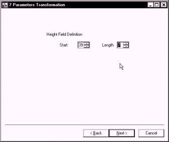
The position of the Height above ellipsoid for the record is entered in the next window.
In our example, the height value starts in column 39 and is 7 characters long.
Please note that for foot-based grids, you still need to enter the height as a metric value. We're working on this, but it isn't ready as of this time.
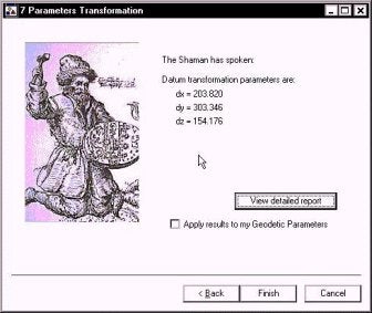
The program then reports the 3-parameter information in the window shown to the right.
If you click the "Apply results to my Geodetic Parameters", then the information is added automatically to your GEODETIC PARAMETERS of the specified MAX project.
If you click the View Detailed Report button, a text report that summarizes the transformation is provided. This also provides residual errors for each of the transformed points.
Datum transformation report

Using geodetic parameters from C:\HYPACK\projects\Macau\Macau.ini
Local ellipsoid is International
Semi major axis: 6378388.000
Flattening:      297.0000000l

Loading C:\HYPACK\Projects\Macau\Internal.txt
6 records meet key criteria
6 records loaded

Geocentric coordinates
----------------------
  -2360868.965    5416590.714    2394336.311
  -2358981.316    5417840.268    2393371.637
  -2360785.882    5418097.292    2391124.776
  -2362644.063    5417436.829    2390916.516
  -2364883.766    5417739.465    2387959.063
  -2362845.969    5419093.046    2387019.007

Loading C:\HYPACK\Projects\Macau\WGS84.txt
6 records meet key criteria
6 records loaded

Geocentric coordinates
----------------------
  -2361072.795    5416287.420    2394182.211
  -2359185.118    5417536.995    2393217.519
  -2360989.678    5417793.911    2390970.578
  -2362847.875    5417133.429    2390762.329
  -2365087.616    5417436.088    2387804.847
  -2363049.798    5418789.694    2386864.767

Performing 3 parameters adjustment...

Datum transformation parameters from WGS-84 to local ellipsoid
--------------------------------------------------------------
dx = 203.820  dy = 303.346  dz = 154.176

Residuals
---------
 0.009
 0.009
 0.002
 0.003
 0.003
 0.004
Cumulative residual: 0.031
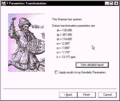
The same routine is followed for computing a 7-parameter transformation. The resulting parameters are reported and can be transferred to the GEODETIC PARAMETERS information as described above.
QHypackにおけるシリアルポートの利用(Serial Port Handshaking)
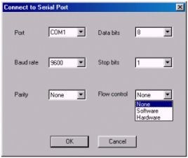
Serial Port Connect Dialog
HYPACK MAXのバージョン00.5は、様々なシリアル機器が対応できるようにハードウェアプログラムをバージョンアップしています。変更の大部分は、目に見えるものではありません。重要なのは次の点です。
HYPACK MAXでは、ハンドシェイク全てがNoneにセットされることが好ましいです。そうすれば、測定が行われると直ちに、それがそれ以上遅れることなくコン ピュータに転送されます。やむをえない理由のない限り、プロッタを除いて全ての装置は、ハンドシェイクに設定しないでください。
あなたの装置にハンドシェイクが必要な場合、その装置がどのようなハンドシェイクのシステムを使うかを決定してください。以下の3つのタイプがあります。
- Xon/Xoff
- CTS/RTS
- DTR/DSR
ハンドシェイクの方法によってシリアルポートのコネクタダイアログで設定するフローコントロールが決定します。そして、場合によってはカスタムケーブルを必要となります。
| Handshaking Method | Flow Control | Cable |
|---|---|---|
| Xon/Xoff | Software | 標準 |
| CTS/RTS | Hardware | 標準 |
| DTR/DSR | Hardware | カスタム |
HYPACK MAXは、シリアル通信ダイアログにおける設定を調整することによって大部分のハードウェアと通信することができます。 そこにまだハンドシェイクのDTR/DSR方法を要求する2、3のデバイスがあります。HYPACK MAXは、通常、CTS/RTSハンドシェイクをサポートしており、それによりコネクティングケーブルの調整が行われることになります。2本のワイヤは、 HYPACKのRTSピンがデバイスのDSRピンと接続し、HYPACKのCTSピンがデバイスのDTRピンと接続するようにしなければなりません。
| HYPACK® | Connection | Device |
|---|---|---|
| RTS |  |
DSR |