FAQ
FAQ検索結果
検索キーワード:
Qローカル・グリッドを設定して測量を行なっている時にSurvey Map画面に表示される船の向きがグリッドと合っていない!
下図のようにローカル・グリッドを回転(Rotation)させた場合、計画測線(LNW)やマトリクス(MTX)はこのローカル・グリッドの設定に基づいて作成されます。
しかし、方位センサからのデータは コンパス方位を出力しているだけです。
<処置> ローカル・グリッドを使用する時には、下図のように方位センサの"Yaw"オフセット(度単位)にもローカル・グリッドの回転角を設定して下さい。
QSBMAXにおけるユーザー定義出力(User Defined Output in SBMAX)[英語]
The Spreadsheet in SBMAX is greatly improved from the one included with the old single beam editor. The primary enhancement is that SBMAX users can configure which data to include in the spreadsheet, and which to exclude. Following that, the selected fields can be exported to a text file for import into 3rd party programs – Microsoft Excel for example. A very simple example of SBMAX user defined output is the topic of this article.
Example
A small experiment is done to find out if any of the GPS quality indicators are useful in detecting bad RTK tide data. The first step is to run a test survey. After that, the files are loaded into SBMAX, where it can be seen in the tide graph that some of the measurements are not quite right.
The SBMAX spreadsheet is configured to include only the values useful to the experiment – GPS quality indicators (DOP, mode and number of satellites) and tide. Configuration is done in View Options, which is accessible by right clicking on the spreadsheet.
The Export button is used for saving to the user defined output file. File is export.txt in the example.
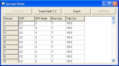
The export file is loaded into Excel.
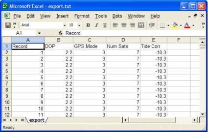
The graph shows that with this GPS set, the only useful quality indicator is GPS Mode. Mode 3 seems to provide good elevation data while modes 4 and 2 are suspect.
Q曳航体用ケーブルの使用(Using a Towfish with the Cable Counter)[英語]
This note briefly describes how to use the cable counter driver to calculate an approximated position for a tow fish.
The cable counter driver can be used either with automatic cable counter devices (currently it supports two formats: Dynapar and MD Totco) or in manual mode (in which case the operator has to update the cable length).
The fish can have either a pressure transducer that outputs the depth of the fish or an altitude transducer that provides the height of the fish above the bottom. Of course it can also be a "dumb" fish without any sensors installed.
In calculating the fish position we make the following assumptions that we know are wrong:
- There is a straight line from boat to fish (i.e. the tow fish is linked using a pole rather than a cable)
- Water depth under the boat and under the fish is the same (you are traveling over an unusually flat bottom)
We have to make these assumptions because otherwise you would have to provide a lot of information regarding the fish and the cable (stuff like drag coefficients, specific weight, etc) and we would have to solve some complicated differential equations. This way, things are a lot simpler for everybody and the only drawback is that the fish might not be where you see it on the screen.
With these assumptions in place the magic layback formula is:

Where
-
Y_offset is the distance from boat's reference point to the A-frame. It is positive when A-frame is astern of reference point.
-
corrected_depth is given by the formula:
corrected_depth = fish_depth + Z_offset
Z_offset is the height of the A-frame above water level and it is positive when the A-frame is above the water (it is cumbersome to place the A-frame under water) - corrected_cable is calculated from the cable length using the following formula:
corrected_cable = catenary_factor x cable_length
It can be seen from these formulas that once user enters a cable length (or we get a reading from the cable counter) we can calculate the layback if we know the tow fish depth. The driver setup box provides four options for determining the fish depth:
- Shallow fish-- the fish depth is always 0 (this is more of a raft than a fish)
- Depth sensor -- the fish is fitted with a pressure transducer that sends out directly the fish depth. You have to interface this device using any of the available echosounder drivers (try using the generic one). You must also configure the mobile associated with the fish to use that device as depth sensor.
- Altitude sensor -- some side-scan sonars provide the fish altitude above the bottom. In this case you have again to configure another echosounder device to provide this information. In addition you have to have a second echosounder that provides water depth for the boat (anyhow it is safer to have an echosounder on board while towing a fish at least to know how deep your diver has to go to rescue the fish). The cable counter driver calculates the fish depth as the difference between the water depth under the boat and the fish altitude (here comes into play that second assumption that the bottom is flat).
- Deep fish - your fish is extremely heavy and hangs straight under the A-frame. In this case the layback is always equal to Y_offset.
A note regarding the offsets set in the "Offsets" dialog box: they represent offsets on the tow fish between the cable anchoring point and the reference point of the tow fish. If you choose the origin of the side scan as reference point on the tow fish and if you care about the difference between the anchoring point and the side-scan origin (after the wild approximation of the rigid pole) than you can enter some values here. However, as a general rule, I would suggest to leave them to 0.
QSurveyプログラムにおけるマトリックスログファイルの使用(Using Matrix Log Files in Survey)
マトリックスログファイルは、マトリックスファイルの集まりです。不規則な調査エリアでは、それによって調査エリアをスペースの浪費を最小限にするいくらかのマトリックスでカバーすることが可能となります。
Surveyプログラムを起動すると、全てのマトリックスは、グレーの長方形(それらのマトリックスが無効であることを意味します)として表示されます。このとき、全てのマトリックスが"Matrix/Display All Matrices." を選択しているのを確認することができます。マトリックスフレームは、赤くなり、全てのセルが適切な色で塗られます。このオプションは、オフラインモードでのみ有効です。加えて、Display All Matricesを無効にせずにオンラインにすることはできません。これの理由は、プログラムにおいて情報の収集が重要である時に、重いグラフィックオペレーション、及び、メモリ割当を持っていることを望まないことによります。
Surveyが オンラインモードで稼働するとき、マトリックスの状態は、船のポジションによって変わります。その間隔がマトリックスに近いならば(そのマトリックス境界 の10%以内)、マトリックスフレームは、青くなります。それは、データ部分がロードされ、更新可能であることを意味します。ローディングプロセスは、個 別のスレッドにあり、測量を中断することはありません。Surveyではいくつかのアクティブマトリックスを持つことができます。しかし、 Viewableにすることができる(赤いフレームで囲まれる)のは一つだけです。その船がマトリックス境界の内部を走行するならば、そのマトリックス は、Viewableになります。この基準(マトリックスのオーバーラップ)を満たすいくつかのマトリックスがあるならば、船に最も近いセンターを持つマ トリックスがViewableとなります。
オフラインモードにもどると、Surveyは全てのアクティブマトリックスを保存し、それらを無効にします。
QSeaBat81XX(サイドスキャンオプション付)のサイドスキャンデータを集録しないようにする
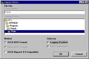
Hysweep Surveyプログラムの起動後に[File]-[Data Logger…]メニューを選択して表示される画面内のSidescan項目、[Logging Disabled]にチェックを付けて下さい。
これによりサイドスキャンのデータ(RSS)を集録しないようになります。
Qインストールに関する注意点(Installing the HYPACK MAX CD-Rom)
古今東西、コンピュータに新しいバージョンのソフトを導入することについては、心配がつきものです。そのコンピュータが測量作業の中心である場合にはなおさらです。我々はMaxのインストールができるだけ簡単になるよう努めてきました。最初に変更したことは、Hypack MaxとHypack 8.9とを同じコンピュータで干渉せずに動作させられることでした。このことによって、現在のバージョンを使いつつ、最新バージョンに触れることができます。測量調査を滞らせるような変更や、不具合が起きることはありません。
私がインストール作業に対して行った変更点を気に掛ける必要はありません。 CDからヘルプファイルや、ワードフォーマットのマニュアル、そしてサンプルファイルもいくつかインストールされます。これらのオプションは、インストール時に除くこともできます。これは我々のソフトウェアの標準的な構成です。
ドングルのドライバに関して注意があります。インストール中にプログラムが動作し、コンピュータ上のドライバを更新します。このプログラムをWindows 95もしくは98で動作させる分には特別な作業は必要ありません。しかし、インストールをWindows NTもしくはWindows 2000で実行する場合には、アドミニストレータの権限を持っていないとプログラムは実行されません。アドミニストレータで再起動すれば、インストールを行うことができます。
ドングルのドライバに関して最後にもう一つ、CDの中にUSBHardlockと名づけたフォルダのことを説明します。このフォルダには、ドングルプログ ラムをさらに更新させるための、単体で実行可能なプログラムが入っています。このプログラムは、ドングルを製作している会社によって更新されます。この新 しいプログラムによってUSBドングルをHypack Maxで使用することができるようになります。これは、このタイプの新しいドングルを使用することのできるHypack のバージョンに限ります。我々が新しいドングルを配布することはまだ可能ではありません。したがって、ソフトウェアがCDにあっても、新しいドングルは将 来的に提供できるであろうとしかいえません。
いつものように、質問があれば東陽テクニカに連絡してください。
Qエラーメッセージ(Class not registered)
QRTK GPSによる潮位補正2(A Discussion of RTK TIDES)[英語]
We have been having a lot of internal discussions regarding the computation of RTK Tide Corrections and their comparison to Measured Tide Corrections. This article presents our current thinking on the subject and illustrates how we are computing and applying the corrections.
1. First – The Basics
The figure to the right shows all of the components needed to compute the Chart Sounding (CS = the distance the bottom is beneath the Chart Datum).
Using conventional survey techniques we have always added the various corrections to the measured depth from the echosounder to obtain the chart sounding. In this example, we have calibrated our echosounder to the surface. The formula would be:
CS = B + T1 + D
CS = 30 + (-10) + 0 = 20.0
where: T1 = Conventional Tide Corr.
B = Measured Sounding
D = Dynamic Draft Meas.
The basics behind the computation of RTK Tide is that we can use the z-value of our GPS antenna to determine the tide correction in real time.
Assuming the vessel is not pitching and rolling (which adds another level of difficulty), we can compute the RTK Tide Correction (T2) as follows:
T2 = -K + N – A + H – D
T2 = -4 + 9 – 22 + 7 – 0 = -10.0
where: K = Height of the Geoid Above the Chart Datum
N = Height of the Geoid Above the Ellipsoid Reference
A = Height of the RTK Antenna Above the Ellipsoid Reference
H = Height of the RTK Antenna Above the Boat Origin Point
D = Dynamic Draft Measurement
The K component comes from an KTD (Kinematic Tidal Datum) file created by the user.
The N component is actually the height of the Geoid Above the Ellipsoid (as read from the Geoid99 model in real time) plus an orthometric correction specified in the Geodetic Parameters program. If the user does not have access to a geoidal model of their area, they should create the KTD file so that it contains K - N values. This would represent the height of the chart datum above the reference ellipsoid.
The A component comes from our RTK system. This is provided anywhere from 1Hz to 10Hz by different GPS systems and broadcast as a part of a GGA or GGK or other message. Every time the KINEMATIC.DLL device driver receives a position update, it computes the new position, along with a new RTK Tide value.
The H component is the static height of the RTK Antenna above the water line. In order to maximize accuracy, this measurement should be taken at the same time you calibrate your echosounder to the surface. In theory, this should be measured to the same point (boat origin = static waterline) that you are using to calibrate your echosounder. In actual practice, it’s not practical to measure the antenna height out in the middle of the channel when you are doing a bar check. It is suggested that you measure the antenna height when the vessel is at the dock and place a mark on the hull to denote the static waterline. Then make an adjustment to the antenna height when you calibrate the echosounder by noting the change in height of the waterline relative to the mark.
The D value represents the vertical movement of the transducer in the water column and is called the Dynamic Draft Measurement. This movement can be caused by a lot of reasons. As you take on more fuel, the vessel can sit lower in the water. Due to squat and settlement, the vessel can have a drastically different position in the water when it is moving that when it is stationary. Some vessels, such as hopper dredges, have pressure transducers that allow us to constantly measure the current draft. Other survey vessels use the DRAFTTABLE.DLL that allows them to construct a table that is used to assign the draft based on the vessel speed. Other survey vessels assume the draft to be a constant and ignore any dynamic effects.
2. Underway – Dynamic Draft Sensor
Now we are driving are vessel over the same bottom that was used in the first example. The tide is unchanged, but due to squat and settlement, the vessel is sitting 1.0 lower in the water column.
Let’s first examine the values that have changed.
A = 21
D = 1
B = 29
All other values are the same.
Computing the RTK Tide:
T2 = -K + N – A + H – D
T2 = -4 + 9 – 21 + 7 – 1 = -10.0
This is correct, as the tide has not changed. Our chart sounding is:
CS = B + T2 + D
CS = 29 + (-10) + 1 = 20.0
In this case, the RTK Tide continues to equal the traditional tide correction (T2 = T1).
3. Underway – No Dynamic Draft Sensor
Now let’s look at the last case again, but this time we do not have any dynamic correction to the draft. We set it for 0.0 (calibrating the echosounder to the surface) and left it there.
Now, the values are the same as in the previous example, except:
D = 0.0
When we compute the RTK Tide (T2):
T2 = -K + N – A + H – D
T2 = -4 + 9 – 21 + 7 – 0 = -9.0
Using the RTK Tide to compute the chart sounding:
CS = B + T2 + D
CS = 29 + (-9) + 0 = 20.0
We still get the correct answer! What you must note (and something I have only recently learned) is that the RTK Tide correction that is computed in this case is not equivalent to the conventional tide correction (T2 ≠ T1).
If we used the conventional approach in this example, the computed chart sounding would be:
CS = B + T1 + D
CS = 29 + (-10) + 0 = 19.
In this case, the RTK Tide result is more accurate than the conventional result. RTK Tides has compensated for the squat and settlement without any measurement of the change in draft. This compensation is built into the RTK Tide value, resulting in it no longer being equivalent to the conventional tide value.
Summary:
The important points of this case are:
When using RTK Tides, you should always calibrate your echosounder to the static waterline.
You should measure the height of the GPS antenna above the water line at the same time you calibrate the echosounder. As a minimum, adjust the GPS antenna height based on the change in draft from when you measured the original antenna height to how the vessel sits during the echosounder calibration.
RTK Tides will generate an accurate chart sounding, whether you apply a real time draft correction or not.
If you apply a real time draft correction, the routine in the KINEMATIC.DLL subtracts the dynamic draft correction in order to compute the ‘true’ tide correction. Absent a dynamic draft correction, the RTK Tide method will still result in an accurate chart sounding, but the user must realize that the RTK Tides values and conventional tide values will not be equal.
If your vessel is prone to squat and settlement or sits differently due to fuel loading, you may want to consider the RTK Tide approach being superior to the conventional tide approach.
QS-57電子海図について[英語]
One of the many changes in the hydrographic field over the past ten years is the use of S-57 for the storage, presentation and transfer of digital chart data. Coastal Oceanographics has been working for several years to be able to present S-57 format files in our HYPACK® MAX and other packages. As a result of this work, we have developed a product to create, maintain and update S-57 chart data.
S-57 is shorthand for Special Publication No. 57, “IHO Transfer Standard for Digital Hydrographic Data”. IHO is the acronym for the International Hydrographic Organization.
The purpose of this document is to provide you with a simple and straight-forward overview of the S-57 format. In other words, this document is sort of like an ‘S-57 for Dummies’ where the intent is to de-mystify how data is stored and managed.
A. Feature and Spatial Data
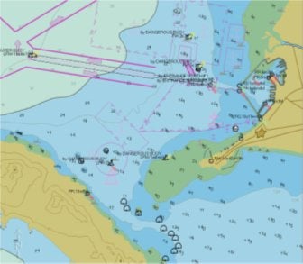
An S-57 file contains digital chart information that is divided into feature and spatial data. A feature is some kind of object, such as a buoy, or a rock, or a traffic separation zone or a light or one of several hundred available objects in S-57. There are point objects (buoys, wrecks, lights, ….), polyline objects (pipelines, cables, roads, ….) and closed polygon objects (depth areas, anchorages, shoreline, …..).
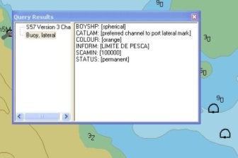
Each feature can be further described by a list of available attributes. For example, the lateral buoy shown in the lower right of the figure contains the following attribute information:
BOYSHP: [spherical]
CATLAM: [preferred channel to port lateral mark]
COLOUR: [orange]
INFORM: [LIMITE DE PESCA]
SCAMIN: [100000]
STATUS: [permanent]
Each attribute is described by a six-letter abbreviation. Thus, BOYSHP = Buoy Shape, SCAMIN = Scale Minimum. Each attribute can require a user entry, a single user choice from a list, or multiple user choices from a list.
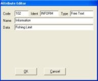
For example: The window to the right is the Attribute Editor for the INFORM attribute. It allows you to enter a single line of text. In this case, we have entered ‘Fishing Limit’.
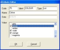
2nd Example: The window to the right is the Attribute Editor for the COLOUR attribute. Note that we can select a single color or multiple colors to describe the object. [In this example, we have the famous brown, violet and orange buoy, used to denote islands inhabited by people with no sense of color coordination.]
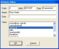
3rd Example: The window to the right is the Attribute Editor for the BOYSHP (Buoy Shape) attribute. In this case, we can only select one item from the available list.
So, a feature tells us what kind of object we have and there are attributes assigned to the feature to tell us some more details. We haven’t yet described where the object is located. That is done with the spatial data.
Spatial data is a fancy way of saying ‘where is the feature located’. In the S-57 format, the locations of objects are described by their WGS-84 positions. Although a user interface might allow you to enter and display the spatial data on a local coordinate system, deep in the bowels of the S-57 file, all the S-57 data is being written as a geographic coordinate (Latitude and Longitude) in WGS-84.
B. Nodes, Chains and Areas
It would have been simpler if they named these Points, Lines and Areas.
One of the favorite buzzwords of an S-57 jockey is ‘chain-node topography’. It’s a fancy way of saying that everything in your S-57 file is either a point (‘node’) or a series of lines (‘chains’). Sometimes the lines form an enclosed shape (‘area’).
A node is a single spatial data point, composed of a WGS-84 coordinate pair. There are two kinds of nodes, isolated and connected. An isolated node represents the position of a point feature, like a buoy or a rock or a wreck. It can’t be used for anything else.
A chain (also referred to by some as an ‘edge’) is a line or a polyline, constructed between two or more coordinate pairs. At each end of the edge is a connected node. We can connect one chain to another by either having them share the same connected node or by making another chain that connects their connecting node with a single line.
An area (also called a ‘face’ by some) is a series of chains (or a single chain) that starts and ends at the same connecting node. In other words, it’s a polygon that describes an area. An area can contain multiple chains (and contain multiple connecting nodes) or can be comprised of a single edge that starts and ends at a single connecting node.
At the top of the adjacent figure is CHAIN 1. This consists of a single line drawn between two connected nodes. This is the simplest of chains.
CHAIN 2 shows a series of coordinate pairs, terminated by connected nodes. This is more typical of an chain.
AREA 1 shows an area constructed from a single chain. It starts and ends on the same connected node.
AREA 2 shows an area constructed from four chains. It is very typical for a area to consist of multiple chains. You can also see another chain (CHAIN 3) taking off from a connected node. This is also very typical, as several features may share the same connecting nodes.
One of the things to keep in mind when you define an area is that as you move along a chain that bounds the area, the enclosed area is always off the right side of the chain.
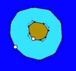
Take a look at the graphic to the right that shows an island (brown), surrounded by a Depth Area (0m to 5m in Light Blue), surrounded by a deeper depth area.
When we create the chain that describes the island as a ‘Land Area’, we need it to go counter-clockwise. That way, the area we are interested in defining is to the right as we traverse around the chain.
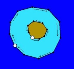
Now take a look at the graphic used to define the Depth Area. We need to define an area with a hole in it. This is done by defining one polygon along the outside and a second polygon along the inside.
Note that the chain defining the outside goes in a clockwise direction, keeping the Depth Area to the right. The chain surrounding the hole (island) travels in a counter-clockwise direction, meaning the depth area is to the right.
Luckily, we can use the same chain to define the Land Area and the inside of the Depth Area. When I select a chain to be used in the definition of an area, I can ‘reverse’ the direction of the chain when used by a particular feature.
C. Combining Features and Spatial Data
The S-57 format stores feature and spatial data as separate records. Each feature record contains information as to what spatial record(s) applies to the feature.
When I want a new buoy to be included in my S-57 file, I first create the buoy ‘feature’ and specify the attributes for the buoy. I then give it the position where I want it to place the buoy. A new feature record will be created that contains the feature type and attribute info. A new spatial record will be created that contains the coordinate point (as an isolated node).
When drawing the S-57 data, it comes across the new buoy in the feature records. It figures out what kind of buoy to draw and what labels are drawn with it from the attribute information in the feature record. The same feature record also contains the location of the spatial record that tells me where to draw the buoy. I open up the spatial record, get the coordinate pair for the buoy and then draw the feature at that location.
This seems a little crazy. Why not just keep the spatial data with each feature record?
One reason for the separation of feature and spatial data is that the same chain might be used for several different features. In our previous example with the island and the depth area, the same chain is used to create the Land Area and the Depth Area. Rather than listing the same set of points for each feature, we save space by only listing the points in one place.
Also, by using this approach, if we change a coordinate pair in the chain used to define the Land Area, we are also automatically changing the coordinate pair used in defining the Depth Area. If each feature had its own set of separate coordinate lists, we would have to make sure that we changed the coordinate pair in every feature’s coordinate list, instead of changing it in only one location in the S-57 scheme.
D. Boundaries and Clipping
S-57 files are ‘bounded’ by two parallels of latitude and two parallels of longitude. The area formed by the bounds is sometimes referred to as the ‘bounding rectangle’. It’s illegal to have any spatial data located outside the boundary area.
In the graphic shown, the top chain would be ‘illegal’, because it contains coordinate pairs that are outside the bounding rectangle.
The lower series of chains forms a legal area. We created it with ‘connected nodes’ along the boundary line, as other features may want to take off from these points.
Some S57 Editors will either automatically clip your chains that pass outside the bounding rectangle while others will just notify you that you have an illegal chain.
Q最新のDXF出力機能について[英語]
The TIN Model program has a new routine for exporting DXF files. While maintaining most of the features of the previous routine, it has a few new features and has become a bit easier to use. You can:
Create labeled contour lines in 1-step instead of creating the lines and labels separately.
Customize contour colors more easily than before. This color scheme is separate from HYPACK® or TIN Model color schemes.
Add weight or texture to a lines to help distinguish them from neighboring contours.
Let’s take a look at how it works and look at these improvements as we go. (We can work from the Sample_Monepts project file, if you have the 2003 HYPACK® Training Conference CD.)
Launch the TIN MODEL program and create a simple TIN to Level model.
Original TIN Model
Access the DXF EXPORT routine in the same way as before, by selecting EXPORT-DXF FORMAT from the TIN MODEL menu.
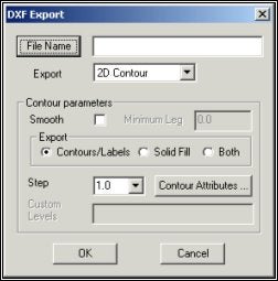
Set your options for the DXF file to be created.
The new DXF Export dialog includes most of the features previously available though you may see them in a slightly different form.
Name the DXF file to be created as you did before. Just click [File Name] and enter the path and name.
The Export Mode is selected from a drop-down list, just a minor change from the former radio buttons.
Note: 3D files only appear in three dimensions when you load them to a CAD program. In HYPACK® MAX, they are viewed from above and appear only 2-dimensional.
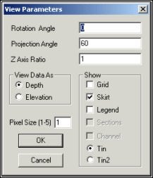
In the previous version of DXF Export, Export Object was selected in this dialog. This selection is now made in the view options dialog.
Most often, you would select TIN. The TIN2 option might be used if you have done a TIN to TIN calculation. In this case, TIN will draw from data in the Input File and TIN2 will draw from the data in the Second File as specified in the Initial Data dialog of the TIN MODEL program.
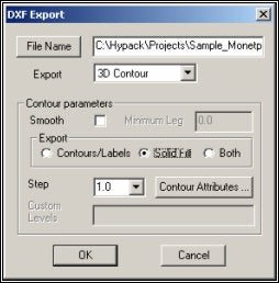
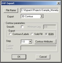
The Contour Parameters area is where the most significant changes have been made.
Smooth enables you to create smoothed contours. It creates a DXF file about ten times the size of the non-smoothed contours. These smoothed contour s can not be plotted from the (older) HYPLOT program. They can be plotted from HYPLOT MAX or from other CAD packages so, if you want to plot smooth contours, you will need a printer that is up-to-date enough to handle it. (Basically, that’s anything other than an old pen plotter.)
The Minimal Leg limits the amount of smoothing. Smoothing will not occur where the TIN Model leg is shorter than specified here. (This option hasn’t changed!)
Export defines exactly how much data should be included.
Contours/Labels creates contour lines and, if specified in the contour attributes, labels for them.
Solid Fill creates color-filled contours.
Both overlays contour lines on color-filled contours.
Step enables you to specify a regular contour interval, used in the creation of 2D and 3D Contours. If you desire an irregular step, click on [Other] then enter your desired contour levels in the Custom Levels field. Leave a single space between each contour level. For example, “2 5 25 100". (This option has only been changed to a drop-down box from radio buttons.)
Once you have the contour parameters set, click [Color Attributes]. The Line and Label Attributes dialog will appear. Each contour level is shown at the left according to the depth range of your data and the Step specified in the previous dialog.
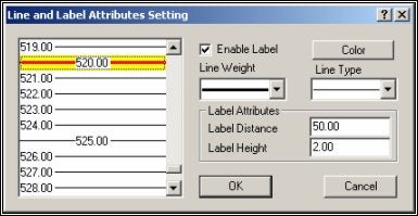
Line and Label Attributes Dialog
You can select one or more of them then, quickly and easily, make selections at the right to set their attributes. The display on the left shows how each contour line will appear in the exported file.
To select several individual contour lines, hold the Ctrl key while you use your mouse to choose your lines
To select a range of contour lines, hold the Shift key and select the first and last line of a range.
Enable Label places labels on the selected contour according to the Label Attributes where:
Label Distance defines the distance, in survey units, between the labels on each contour.
Label Height sets how big the label will be.
Line Weight offers a choice of increasing thicknesses for you to accentuate certain contours.
Line Type provides five options, solid line and four combinations of dots and dashes for further distinction from other lines.
Note: Windows® can not handle both line type and weight. Therefore, in any Windows® application, including HYPACK® MAX, contours that have been given both a dotted line type and a weight thicker than 1 pixel, will appear solid. They will, however, be drawn with both type and weight characteristics if you import them into a CAD package.
In this example, we have created contours every foot (or meter depending on your survey units) and every 10th contour is accented with a weighted red contour line. Also, every 5th contour is labeled at 50 foot (or meter) intervals along its length with numbers 2 feet (meters) tall.
When you have finished specifying contour attributes, click [OK] to return to the DXF Export dialog.
Click [OK] again to create the DXF file. You will see the file drawn to the TIN screen.
It will be saved to the specified place and File Name ready to be loaded to HYPACK® MAX as a background file or to any other package that uses DXF format files.
Resulting DXF File drawn to HYPACK® MAX screen
In this example we created 2-dimensional,
labeled contour lines.
With one or two simple changes in the DXF Export dialog,
we can make it 3-dimensional file or
a solid fill contour.
Close up View of Resulting DXF in HYPACK® MAX
Change the Export Contour Parameter to “Solid Fill” and the lines and labels are replaced by a color-coded solid image.
Solid Filled Contours
Change the Export Contour Parameter to “Both” and the labeled contour lines are superimposed on the solid fill model.
Smoothed, Solid-filled, Labeled Contours
Q曳航体等の使用(New Developments in the Hardware Setup for Mobiles)
Hardwareプログラムで曳航体などの装置をしようする場合のセットアップ方法を以下に示します。 どのような曳航体を使用する場合でもOffsetダイアログにおける左舷、右舷のオフセット値は通常オフセットを入力する場合に対し、符号を反転して入力しなければなりません。
| 計測方向 | 通常の場合 | 曳航体の場合 |
|---|---|---|
| 左舷方向 | マイナス | プラス |
| 右舷方向 | プラス | マイナス |
浚渫機のホッパーアームも曳航体の場合と同様です。
以下の例では3タイプの機器について説明しています。T
曳航体と単純な曳航経路計算
 |
Devices | Dialogs | |
|---|---|---|---|
| Driver Setup | Offsets | ||
| GPS | 右舷 -5 前方 -5 アンテナ高 |
||
| Cablecnt.dll | Y オフセット -20 Z オフセット = 水面からの高さ |
右舷 -5 前方 0 高さ 0 |
|
| Towfish | 右舷 0 前方 -10 |
||
ケーブル繰り出し長はSurveyプログラムで制御されます。
注意: この例の場合、 Cablecnt.dllの以下の設定を使用することで補正されます。
| Devices | Driver Setup | Offsets |
|---|---|---|
| Cablecnt.dll | Y オフセット 0 Z オフセット = 水面からの高さ |
右舷 -5 前方 20 高さ 0 |
トラックポイントシステム
|
Devices | Dialogs Offsets |
|---|---|---|
| GPS | 右舷 -5 前方 -5 アンテナ高 |
|
| Trackpoint | 右舷 -10 前方 20 高さ 0 |
|
| トラックポイントシステムではダイレクトに曳航体のポジションが出力されるため曳航体のオフセット値を入力する必要はありません。 | ||
 |
Devices | Dialogs Offsets |
|---|---|---|
| Hopper Arm #1 | 右舷 12 前方 -10 |
|
| Hopper Arm #2 | 右舷 -4 左舷 10 |
Qデータ変換(Datum Transformation – Field Example)
マカオ島で使用するのに適切なデータム変換値を必要としている香港の代理店(Steve Lai)から、最近、以下の情報を得ました。
| Station Name |
Geographic Coordinates (WGS84) |
Projection Coordinates |
|---|---|---|
| Hotel Oriental | Lat. N22 – 11 – 32.6903 Lon. E113 – 33 – 12.2133 Ht. 73.854 |
East 21436.566 North 17920.459 MSL 76.13 |
| Monte Da Barra | Lat. N22 – 10 – 58.8428 Lon. E113 – 31 – 54.3789 Ht. 72.119 |
East 19207.44 North 16878.29 MSL 74.46 |
| Taipa Pequena | Lat. N22 – 09 – 39.4636 Lon. E113 – 32 – 48.5433 Ht. 109.680 |
East 20760.29 North 14437.4 MSL 111.97 |
| Taipa Grande | Lat. N22 – 09 – 31.5112 Lon. E113 – 33 – 57.2049 Ht. 158.185 |
East 22727.683 North 14193.896 MSL 160.36 |
| Monte Ka-Ho | Lat. N22 – 07 – 48.0785 Lon. E113 – 35 – 04.6180 Ht. 130.037 |
East 24661.59 North 11013.768 MSL 132.06 |
| Coloane Alto | Lat. N22 – 07 – 14.5545 Lon. E113 – 33 – 40.5583 Ht. 170.316 |
East 22253.264 North 9981.001 MSL 172.41 |

Geodetic Parameters set to Macau.
初めにしたことは、HYPACKで地理座標パラメータをマカオ座標にセットすることでした。マカオ座標は国際座標の一つであり、Grid menuリストから選択する事ができるので、とても簡単にできました。
右図のGEODETIC PARAMETERSプログラムの通り、マカオ座標は国際地球楕円体に基づいています。GPSからの緯度経度情報はWGS-84なので、SURVEYプロ グラムは、緯度経度を、投影座標に落とす前に、マカオデータムに基づいた国際地球楕円体の緯度経度へデータム変換計算を行っています。
右図について、Datum Transformation parameters are setの項目は0.00にセットされています。まだ、どんな値を入れるべきか決めていないからです。
次にすることは、緯度経度をマカオデータム(国際地球楕円体)の投影座標へ計算することです。これはGrid Conversionプログラムを用いて行います。XY to Geographicsボックスにチェックをいれます。そして、各々のX-Y座標を入力します。各々の座標に対するローカルな緯度経度が出力されている、中央のウィンドウ中の値を記録します。
さて、これで各々の座標に対する、WGS-84(GPSから与えられている)の緯度経度と楕円体高度と、マカオデータム(国際楕円体)における緯度経度、平均海水面からの高度が判りました。
平均海水面からの高度よりも、マカオデータムからの楕円体高度が判る方が望ましいのですが、今わかっている値で話を進める事にします。
次に、Datum Transformationプログラムを用いて、平行移動3-パラメータを決定し、各座標について比較を行います。左図は、Hotel Orientalにおける変換です。各々6点における平行移動量を決定しました。以下にまとめます。
| Station Name: |
DX |
DY |
DZ |
|---|---|---|---|
| Hotel Oriental |
204.52 |
203.95 |
155.09 |
| Monte Da Barra |
203.95 |
303.34 |
154.19 |
| Taipe Pequena |
203.08 |
302.74 |
154.88 |
| Taipe Grande |
203.13 |
302.40 |
155.66 |
| Monte Ka-Ho |
201.98 |
301.56 |
156.46 |
| Coloane Alto |
201.41 |
301.71 |
155.50 |
| Average Value: |
203.01 |
302.49 |
155.30 |
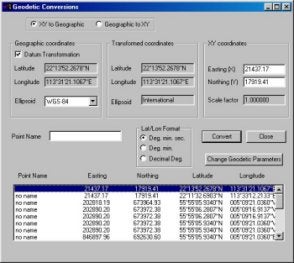
Determining the Lat/Long on the Macau datum.
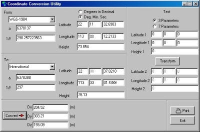
Determining the 3-parameter shift at Hotel Oriental.
完璧であれば、6つの各ステーションに対する平行移動3-パラメータの差異は数センチ以内になります。本例のように完璧ではない場合、数メートル程度の差異がでます。この原因としては、
- 誤ったWGS-84情報
- 誤ったマカオデータム緯度経度
- マカオデータム情報に基づいた楕円体高度の替わりに、MSLからのエレベーションを使用している
水路測量者には、3つの選択肢があります:
- マカオでの測量全体に対する平均値を用いる。
- 各々の点に近い点に対する最も適切な値を用いる
- 3-パラメータの使用をやめて7-パラメータを用いる
選択肢 #1: 島全体に対する平均値を用いる
WGS-84の緯度経度高度から、全てのステーションの情報をマカオデータムへ変換し、そして投影座標へ計算させました。計算されたステーションの座標と、実際の座標とを比較して、位置誤差がどの程度になるのか見積もりました。結果は以下の表にまとめられます:
| Station Name: |
D Easting |
D Northing |
|---|---|---|
| Hotel Oriental |
+1.67 m |
+0.22 m |
| Monte Da Barra |
+1.19 m |
+1.18 m |
| Taipe Pequena |
+0.16 m |
+0.47 m |
| Taipe Grande |
+0.07 m |
-0.37 m |
| Monte Ka-Ho |
-1.32 m |
-1.24 m |
| Coloane Alto |
-1.78 m |
-0.21 m |
上表から、全てのデータム変換に対する平均を用いた場 合には、Easting方向は最大1.78メートルの誤差 (ステーション:Coloane Alto)、Northing方向では1.24メートルの誤差(ステーション:Monte Ka-Ho)が現れました。縮尺1:5000において、この誤差は0.3mmの大きさで表示されます。この誤差が許容範囲か、そうでないか微妙なところです。
選択肢 #2: 各々の点に近い点に対する最も適切な値を用いる
この場合、Hotel Orientalに近いところを測量しているならば、平行移動パラメータは、この地点における平行移動パラメータを入力します。Coloane Altoに近い場所ならば、 そこの地点のパラメータを入力します。これにより、各々の地点における正確な値が得られます。しかし、その地点から離れるにしたがって値は正確ではなく なっていきます。どのくらい値が悪くなるのかといいますと、上記の例では、Coloane AltoとHotel Orientalは約8km離れていますが、Hotel Orientalでの値を用いてColoane Altoまで移動すると、位置誤差はEasting方向で3.45メートル、Northing方向では0.43メートルになります。つまりHotel Orientalから1kmごとに0.45メートルの誤差が出てくることになります。
選択肢 #3: 7-パラメータを用いてデータム変換をする
与えられた情報を元に、エリア全体を精密にモデル化した7パラメータを用いた変換を行うことができます。通常、7パラメータデータム変換を行うには7もし くはそれ以上のテスト地点が必要となります。HYPACKには、この機能がないので、商用の他のソフトウェアを用いて行わなくてはなりません。
QSBMAXのデータ比較機能(SBMAX Vertical Comparisons)[英語]
SBMAX is the new single beam editing program. It has been available for beta testing for a while and will be the default editor of the Hypack® Max version 2.6 release. SBMAX has many useful features, one of which is to graphically compare vertical data provided by the echosounder, heave compensator and even water levels from RTK-GPS sets.
The following examples are from survey data courtesy of the USACE Seattle District.
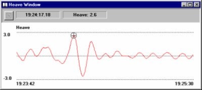
Heave Window
This is simply a time series of boat heave measurements. The cursor may be placed anywhere upon the graph to find the measurement at that point in time. In this example the small boat experiences a moderate have of +/- 3 feet.
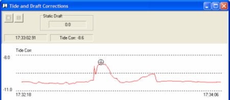
Tide Window
The tide and draft corrections window (below) shows raw RTK tide measurement in blue and processed tide measurement in red.
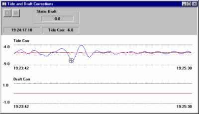
Correlation of the cursor position between and tide and heave graphs shows a minimum tide value at a maximum heave value. This is right because heave is shown positive upward and the tide correction is positive downward. The fact that the min/max points align indicate that GPS latency has been correctly applied.
The red line shows the tide correction that is actually applied to the raw soundings. It is derived by averaging raw tide measurements over 30 second intervals. Without this modification to the raw RTK tide measurement, heave would be doubly corrected, which is never a good thing.
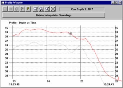
Profile Window
The Profile Window is where all corrections are tied together. The red line is the corrected soundings, the gray line is uncorrected and it is easy to see the effect of the corrections. For example, the dip in the uncorrected depth at the cursor position is clearly the result of the boat heaving upward, and is not apparent in the corrected depth.
The cursor position reflects the time of the heave and tide corrections described above.
Conclusion
The increased graphical capabilities of SBMAX allows analysis of survey data never before available to Hypack® users. All you stuck on Hypack® 8.9 – What are you waiting for?
Qデジタイザによる測深値の入力(Using The Echogram Program)
ECHOGRAMプログラムは、測深データをマニュアルでディジタル化するために使用します。ディジタル化された測深値は、SINGLE BEAM EDITORプログラムで処理されるデータと結合処理することができます。
このプログラムは、あなたが使用しているディジタイザに付属するウィンドウズディジタイザドライバを利用します。
いったん、あなたがご自分のディジタイザドライバをインストールすれば、メニューよりUtilities-Digitizing-Echogramを選択し、 Echogramプログラムを実行が可能になります。
ダイアログ・ボックスは、あなたがポインティングデバイスの第4のボタンを押すことによってあなたのディジタイザの機能を停止することができるメッ セージを表示します。OKボタンをクリックするとECHOGRAMプログラムが起動します。メニューのDIGITIZERより使用中のデジタイザの有効・ 無効が設定できます。
メニューよりChart-Scaleを選択します。
あなたのチャートと一致するMinimum Depth、及び、Depth Range (数字1を見る)をテキストボックスに入力し、OKをクリックします。
図2 :チャートを記録するために、ウィンドウの下部の指示に従ってください。
メニューよりChart-Register Chart選択します。すると、ディジタイザをチャートの上端と底辺中心に置くようにメッセージが表示されます。
いったん、あなたがこれらのポイントを入力すると、チャートで最初に入力するポイントを要求するダイアログ・ボックスが表示されます。チャートから最初のポイントを入力し、そして、OKをクリックします。
すると、位置マークをディジタル化するように促すメッセージが表示されます。各々の位置をディジタル化するために、最初のボタンをクリックします(図3を参照)。左から右に処理し、終了するときは、2番目のボタンをクリックします。
図3 :固定点をディジタイジング
図4 :測深値をディジタル化する
全てのポイントの位置を入力し終わると、プログラムは、測深値をディジタル化し始めるようにメッセージを表示します。左からスタートし、測深データを入力していきます。 (図4を参照)。終了時はディジタイザの3番目のボタンを押します。1番目のボタンを押すことによって再び入力することができます。
入力がすべて終了したら、File-Save Asを選択し、名前を付けて保存します。ファイルは、*.depの名前で保存されます。
この*.depファイルは、ASCIIフォーマットファイル保存されています。
サンプルを下記に示します。:
| 109.04 | 17.27 |
| 109.09 | 17.35 |
| 109.11 | 17.44 |
| 109.15 | 17.55 |
| 109.19 | 17.58 |
| 109.18 | 17.73 |
| 109.20 | 17.70 |
| 109.27 | 17.85 |
| 109.30 | 17.91 |
| 109.37 | 18.06 |
最初のカラムは、測深データの水平位置を表し、第2のカラムは、その位置のディジタル化された深さを表します。
Qフィラデルフィア法体積計算結果について(Philadelphia Pre- and Post-Dredge Reports)[英語]
There have recently been a lot of questions as to the meaning of items in the Philadelphia Pre-Dredge and Post-Dredge Reports of the CROSS SECTIONS program. The purpose of this article is to examine those items and to provide an explanation of differences between the Pre-Dredge and Post-Dredge numbers. I ran the Philadelphia Pre-Dredge method using a Before-Dredge (befores) and an After-Dredge (afters) data sets. I then ran the Philadelphia Post-Dredge method using both data sets.
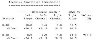
Philadelphia Pre-Dredge Report - Befores
Let's first take a look at a section of the Philadelphia Pre-Dredge Report. If you get down to the station-by-station numbers, you'll see something like the following for your data set:
For the Station 0+10, the Left Slope has 20.0m² of material; the Left Center Channel has 13.8m² of material; the Right Center Channel has 8.6m² and the Right Slope has 15.3m².
The Offsets refer to the distance (from the centerline) to each feature. The Top of the Left Slope is -66.5m (left 66.5) from the centerline; the Left Toe Line (start of side slope) is -51.5m (left 51.5); etc.
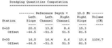
For the Section 0+30, the information is repeated. Since our lines in this test are 20m apart, we can create a simple table to determine the volumes for each section. Volume = (Area1 + Area2) * Dist / 2.
| Section/Area | Left Slope Area | Left Channel Area | Right Channel Area | Right Slope |
|---|---|---|---|---|
| 0+10 | 20.0m² | 13.8m² | 8.6m² | 15.3m² |
| 0+30 | 16.5m² | 16.4m² | 6.6m² | 13.6m² |
| Volume | 365m³ | 302m³ | 152m³ | 189m³ |
| Total Volume | 365 + 302 + 152 + 189 = 1108m³ | |||
The difference between the report's 1106.7 m³ and the 1108 m³ in our table is that the areas in the report are only reported to 0.1 precision but are maintained at a higher precision inside the program.
The same can be repeated for the numbers in the Overdepth area of the report. These numbers are located in the right-hand side of the report and contain the areas and volumes of material in the Overdepth area.
Philadelphia Pre-Dredge - Afters
I then ran the data files from the After-Dredge survey, using the same Philadelphia Pre-Dredge report. This will be handy later on when comparing numbers in the Philadelphia Post-Dredge Report.
In this case, if I repeat the computation done above, I get the volume between the two sections to be 736 m³. This is almost equal to the value in the report, the difference being that I am using the areas that have been rounded to the nearest 0.1m².
So far, so good.
Philadelphia Post-Dredge Report - Befores and Afters
Now let's take a look at the report from the Philadelphia Post-Dredge method.
There are two sets of "areas" reported for each section.
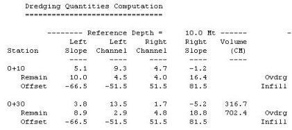
The top line (5.1 9.3 4.7 -1.2) represents the amount of material (m²) that has been removed in each segment. It determines this number by first determining where the two data sets overlap. It then computes the available area in Survey 1 (S1) and the available area in Survey 2 (S2) and computes the area of material removed (S2-S1). The negative number (Right Slope) in our example reflects that material has actually been added in the Right Slope area in the area of comparison.
The second line (10.0 4.5 4.0 16.4) represents the amount of material that is still available in the section. You will notice that these numbers are slightly different than those reported at the top of the page in the Philadelphia Pre-Dredge report using the After-Dredge data (10.0 4.5 4.0 17.5). The reason for that is that the Philadelphia Post-Dredge will only report area where there is overlapping data on both surveys. [This is also true for the material that has been removed.]
Let's take a close look at the pre-dredge and post-dredge sections for line 0+10.
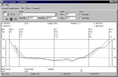
If we take a close look at the right side slope (the area from 51.5 to 81.5 on the right of the graph), the line from your before-dredge survey is displayed in black and the line from your after-dredge survey is displayed in blue. The black line stops right at the 5.0m level. For the Philadelphia Post-Dredge method, all area computations will stop at this point for both surveys. (Even though there is information in the after-dredge survey that is not going to be used.)
The post-dredge line originally reported 17.5m² of area available on the Right Slope in the Philadelphia Pre-Dredge report. In the Philadelphia Post-Dredge report, there is only 16.4 m² of area available. This is because it has not included the 1.1 m² of material that occurs beyond the point where the before-dredge survey ended.
Looking again at the Philadelphia Post-Dredge Report:
The value of 316.7 m³ reflects the amount of material that was removed between station 0+10 and 0+30. Once again, this is only computed where both data sets overlap.
The value of 702.4 m³ is the amount of material that remains to be removed (once again where we compare only areas where the two data files overlap).
In the Philadelphia Pre-Dredge report (using the after-dredge data file), it reports 735.3 m³ of available material. We have lost 32.9 m³ because the before-dredge survey did not overlap all the way across with the after-dredge survey. Note: If the after-dredge survey did not extend all of the way across and the before-dredge did extend all of the way across, the reported volumes in the Philadelphia Post-Dredge report would also be smaller than in reality.
If I take the available material generated by running the before-dredge and after-dredge surveys (separately) through the Philadelphia Pre-Dredge report and take the difference, I get 371.4 m³ (1106.7 - 735.3), versus the 316.7 m³ reported above.
Which value is correct? They are both correct. It is just that the Philadelphia Post-Dredge method is designed to only compare areas where there is over-lapping survey data.
Note: The Average End Area 3 method handles things differently. It computes all of the area under the pre-dredge survey and then computes all of the area under the post-dredge survey and then takes the difference without worrying about where the two data sets overlap. This is the major difference in the reported quantities between the two methods.
Philadelphia Post-Dredge Report - Summary
Finally, lets take a look at the Philadelphia Post-Dredge Report.
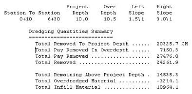
The top item is Total Removed To Project Depth. This is a sum of all of the material removed above the design template. It is computed by adding all of the reported quantities in the report. It would take the quantity between lines 0+10 to 0+30 (316.7 m³) and add it to the quantity between lines 0+30 to 0+50 (265.1 m³) and add it to the quantity between lines 0+50 to 0+70 (187.3 m³), etc.
The item Total Pay Removed In Overdepth is the sum of all of the material reported removed between the design template and the over-depth template. It's the same as above, repeated using the "over-depth" numbers in the right hand side of the report. (173.9 + 163.7 + 129.9 …..)
The Total Pay Removed is the mathematical sum of the above two item.
The Total Removed is the Total Pay Removed plus the material removed beneath the Overdepth template. In our test case, we have actually added material beneath the Overdepth template, so the Total Removed is less than the Total Pay Removed. There are no numbers in the report to confirm this. You can only examine the sections in the areas where the depths are less than the Overdepth template. It's very useful to plot out both sections on top of each other. Please look at the section below.
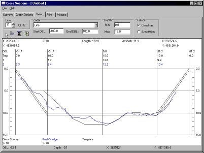
If you take a look in the area where the data is deeper than the over-depth template (center channel), the before-dredge survey (black) is deeper than the after-dredge survey. In effect, there is now more material in the center of the channel, although it is still beneath the over-depth template. This is what is causing our Total Removed to be less than our Total Pay Removed. This happens very rarely.
The Total Remaining Above Project Depth is just the sum of all of the remaining volume quantities for each pair of sections from the report below. In our case it would be 702.4 + 671.9 + 469.4 +…..
The Total Overdredged Material is the mathematical difference between the Total Removed minus the Total Pay Removed. Normally, it is used to show how much extra material the contractor removed beneath the over-depth template. Since we get a negative, it shows how much material has accumulated beneath the over-depth template in your project.
The Total Infill Material is the sum of all material where the pre-dredge survey was deeper than the post-dredge survey. There are no specific numbers provided in the report to verify this number.
Qハードロックキー、ドングルに関するエラー(HARDLOCK, Keys & Dongles)
ハードロックが故障したと思われる場合、別のコンピュータでテストした後で以下の点をチェックしてみてください。
全てがだめだった場合、
- あなたのシステムbiosでパラレルポートのモードを「NORMAL」か「UNIDIRECTIONAL」(EPP-ECP-双方向のBAD )に切り替えてください。
- HPの双方向プリンタドライバを取り除きます。
- プログラムを監視するあらゆるHPを取り除きます。
- あなたの電源管理設定を消去します。
- autoexec.batにおいてこのラインを試みてください。
Set hl_search=278i,378i,3bci, - ある会社(COMPAQや東芝などを一例としてあげれば)は、それらのOSとしてWin9x専用のフォームバージョンをロードし、パラレルポートの認識を不能にすることが有ります。その場合には、ディスクをフォーマットして正規の古い01バージョンからWIN9xをロードしてください。
- あなたはのお持ちのハードロックは、おそらく不良品か故障しています。
- 新しいパラレルポートのカードを入手します。
- USBポートをお持ちなら、我々のUSBキー(99年5月以降利用可能なもの)のうちの1つを試みてください。
- おそらく、ISAまたはPCIスロットを占める内部のキーを得ることができるでしょう。
- 最終選択:新しいもしくは別のコンピュータを入手してください。
Qデータのコピー(Hypack/Windows Interfacing Tips)
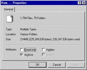
今日、CD-R、CD-RWなどのデータ保存方法が一般化してきています。一度これらのメディアにデータを書きこんだ場合、これらのデータはすべて読み出し専用となっていることに注意してください。
CD-Rなどにバックアップしたファイルを再び利用するには以下の操作を行います。
- コピーしたファイルを右クリックし、メニューよりプロパティを選択します。
- プロパティウィンドウの属性欄の読み取り専用のチェックマークをはずします。
以上でHypackで編集が可能となります。
QSurveyプログラムのリモート操作(Remotely Controlled Survey)[英語]
Imagine you have to perform a survey with one small vessel that is big enough to accommodate pilot and necessary surveying equipment (GPS, echosounder, motion sensor, Left Right indicator, laptop computer).
Obviously, the small vessel is not spending much fuel, it moves easily, does not require any additional crew member. Unfortunately, there is not enough space for somebody to concentrate on the surveying business.
The possible answer is remote surveying with an additional survey unit located on nearby bigger vessel or in a car along the shoreline. The current version of HYPACK® supports such a situation. It requires additional hardware (one computer, two radio modems, one additional comport for moving unit) and software (two device drivers).
The operator on the Moving Unit can see only the left/right indicator and eventually the on/off line signal. His goal is to keep the left/right position as close to the center as possible. The surveyor in the Stationary Unit receives positions from the Moving Unit and makes the decision to start/suspend/end the survey. Every event ( start/end survey, switch/swap line) on the Stationary Unit is forwarded to the Moving Unit and interpreted by the output device driver.
It is important to note that the Moving Unit receives and saves all surveying data. The question is would it not be cheaper to get rid of HYPACK® on the Moving Unit and send all data by radio modem to the Stationary Unit.
Obviously, it is cheaper but we are going to make the radio modem very busy and that can result in loosing some data. Additionally, the operator on the Moving Unit is not going to have a left/right indicator position which might cause wasting of surveying time.
Q古いペンプロッタを使用した場合の不具合について(Hyplot Contours and Pen Plotters)
HyplotプログラムでDXFコンタファイルを出力したときにコンタラインが点集合でプロットされることがあります。これはプロッタがHP/GLをサポートしていないために発生する現象です。 このの現象が発生した場合、Hyplotプログラムのパラメータ設定ダイアログでsmoothness値を設定してみてください。
Smoothnessパラメータを設定すると、各々の点がスプラインで結ばれ、スムーズのコンタが出力されるようになります。 この設定は特にHP/GL2をサポートしたプロッタで有効です。
TinモデルプログラムでDXF出力をするときに "Smooth Contours"をチェックすることでもスムーズなコンタを作成することができます。
Q複数のコンピュータでのターゲットの同期機能について(Target Synchronization Driver)[英語]
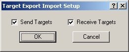
A new device driver, “tgtexportimport.dll”, has been developed to provide target synchronization between two separate computers running Survey. You can set whether each computer will send or receive targets, or do both.
The computers can be connected by either a serial or network cable.
Serial Connection: The communication settings should be identical.
Network Connection: One computer is designated as the server and the other as the client.
Once the connection is established every target created on one computer will be echoed on the second computer.