FAQ
FAQ検索結果
検索キーワード:
Q共有メモリ(Shared Memory Programs)[英語]
Memory from the Shared Memory area running with Survey
The release of HYPACK MAX brings a new feature with the SURVEY program call "Shared Memory". Developed by Craig Berry and Lazar Pevac, this new feature allows the SURVEY program to make its information available to other programs operating on the same computer. HYPACK can now share the navigation and targeting data with other applications. Already the MULTISCAN program which provides real time visualization of multibeam and side scan sonar data has been adapted to make use of this feature. Ocean Imaging which makes the GeoDAS side scan sonar and multibeam visualization/targeting program has also adapted their software to be able to get their information through this shared memory area.
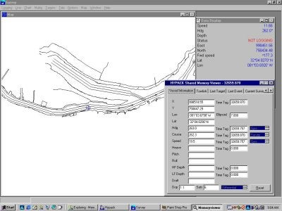
"Shared Memory" is a special area in RAM which the SURVEY program can post the latest information. Every time there is a navigation update, the WGS-84 Lat/Long/Ht, local datum Lat/Long/Ht, project X-Y, Hdop, # of Satellites, time tag and other relevant information are posted to the shared memory area. The same is true with depths, tides, heave-pitch-roll, ROV and towfish position and just about any other information relevant to HYPACK. Other applications can access this area for their survey information as fast as they require.
What’s nice about this new feature is that it allows us to write small custom programs without have to make changes to the SURVEY program. For example, in the application to the right, Craig has made a small program which displays the values for the vessel and ROV from the shared memory area. It also contains a graph of the HDOP and # of Satellites. This is a stand-alone executable, meaning it does not effect the SURVEY program in any way.
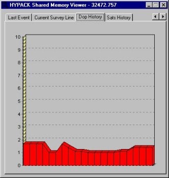
HDOP graph from Shared Memory area.
Already we have created a special program which reads the displayed memory area and allows you to select which items you wish to export, what order you wish them exported, how often to export them and which port to export them over. This will replace a lot of the custom output drivers we have had to develop in the past. We are also building a barge monitoring program which takes the information from the SURVEY program and records it to a user-requested file format. It is a lot faster and more cost effective for us to write a short executable rather than have to try to adapt the SURVEY program to meet everyone’s needs. It also is safer, as we don’t have to mess with the SURVEY program while we try to meet user’s requests.
Q測深値の補正(Sounding Adjustments Program)
SOUNDING ADJUSTMENTSプログラムは編集済みのAll Format形式のログファイルに対して音速補正を施すアプリケーションです。補正処理終了後の結果は、single bean editorのSV correction columnを参照する事で確認出来ます。
- PROCESSINGメニューからSOUND VEROCITY-SOUNDING ADJUSTMENTSをクリックして、音速補正プログラムを起動すると、水深、音速入力テーブルが表れます。
- テーブルの各項にデータを入力してください。水深値の単位はgeodetic distans unitsで指定した単位と同じです。Correctionの単位はm/secです。
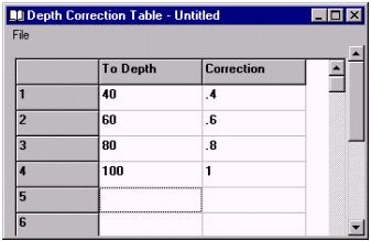
Depth Corrections Table - 作成したテーブルの保存は、FILEメニューからSAVE又は、SAVE ASで名前を指定して行ってください。
- FILEメニューからGENERATEを選択し、ログファイルに対して補正を行います。SINGLE BEAM EDITORにより補正の結果を確認することが出来ます。このサンプルシートでは、水深40m以下は0.4、40mから60mの間では0.6が採用されます。
Qクロスセクションでライン(LNW)ファイルを利用して体積計算する

この例で計算に使用されるチャネルは、上の図において示されるものです。A-B-D-C-A多角形の中に含まれるエリアは、深度8.0mにあり、A-B toeラインから0.0mに達する10:1のサイドスロープがあります。同様に、C-D toeラインから0.0mに達する10:1のサイドスロープがあります。
Tin Modelプログラムで断面を切る
Tin Modelプログラムで断面を生成するにはあらかじめ測線(*.LNW)ファイルを作成しておく必要があります。
TIN MODELプログラムを起動します。初期設定の第ログでInvert Z ValuesをチェックしZ値を反転させます。Section File欄にあらかじめ作成した測線ファイルを入力します。その他の設定は通常Tin Modelを作成する場合と同様です。
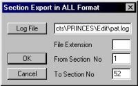
Export – All Formatを選択します。Log File欄に作成する断面のファイル名を入力します。このルーチンは、各測線に毎にHYPACKのAllFormatのデータファイルを作成し、それを現 在のプロジェクトの/Editディレクトリに保存します。
各ラインは、例えばcenterline (に沿ってそのラインに基づく名前で保存されます。(‘0+00’、‘2+00’、‘4+00’、…):
|
ライン名 |
ファイル名 |
|---|---|
|
0+00 |
0+00.ALL |
|
2+00 |
2+00.ALL |
|
4+00 |
4+00.ALL |
|
…… |
………… |
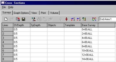
TIN MODELプログラムを終了し、CROSS SECTIONSプログラムを起動します。Surveyタブにおいて、Tinモデルで作成された断面のカタログファイルの名前を入力します。するとカタロ グが含むファイルが読み込まれ、図において示されたように、順番にそれらをリストされます。同じく0.5mの余掘り値を入力し、計算方法としてAEA1 Methodを使うように設定します。
その結果生じる断面は、下のスクリーンキャプチャにおける14+00の間で示されます。
ボリューム量の要約は、下図で示されます。
以下に示される表は各計算方法による結果の比較です。
|
ケース1 :Tin ModelにCHNファイルを使用 |
2,522,802.5 m³ |
|---|---|
|
ケース2 :Tin ModelにLNWファイルを使用 |
2,517,678.5 m³ |
|
ケース3 : CROSS SECTIONSにTin Modelで生成された断面を使用 |
2,500,658.5 m³ |
この方法で計算を行うと他の2つの計算結果に比べ17,000 m³(約0.7%)少ない結果となっています。
おそらく、この差異は、いくつかのラインのエンドの水深データの希薄なデータが存在することによると思われます。
上図は、2、のラインのために作成された水深測量を示します。
TIN MODELは、TIN三角形の脚が測線(ライン)と交わる全てのロケーションで測深データを作成します。ラインがスロープのトップを越えて伸びていない場 合、ラインエンドでギャップから時折離れたものとなります。(ライン端の直下の基準面の深さを採用します。)これが原因で体積計算の際の誤差となることが あります。
ラインを延長して再計算した結果は下記の通りです。:
|
左サイドスロープ: |
30,772.7 |
|---|---|
|
チャネルの中心: |
2,420,966.5 |
|
右サイドスロープ: |
68,232.5 |
|
計画水深に対する体積: |
2,519,971.7 |
結果は、非常に首尾一貫したものとなりました。:
|
ケース1 :Tin ModelにCHNファイルを使用 |
2,522,802.5 m³ |
|---|---|
|
ケース2 : Tin ModelにLNWファイルを使用 |
2,517,678.5 m³ |
|
ケース3 : CROSS SECTIONSにTin Modelで生成された断面を使用 |
2,519,971.7 m³ |
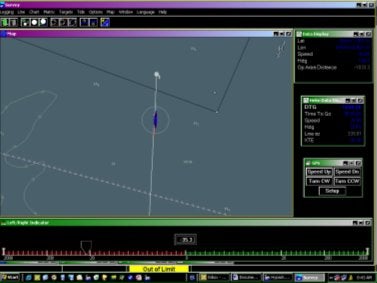
Qリアルタイムプロット機能(Real Time Plotting in Survey)
測量中、Surveyプログラムは、リアルタイムに航跡、及び、測深値をプロットすることができます。航跡はボートエディターでボートを作成した際の基点を基準に描画されます。バージョン7.1ではユーザーは、Plotter Setupダイアログによってプロッタの設定を行います。8.1以降のバージョンでは、HardwareプログラムでHP/GLデバイスドライバを選択します。
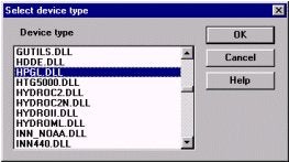
Figure 1: Selecting the plotter driver in Hardware
プロッタは、航跡をリアルタイムでプロットするにはHP/GL互換機を使用しなければなりません。インクジェットプロッタやレーザジェットプリンタも使用可能ですが、航跡のリアルタイムプロットは実行できません。
プロッタドライバをインストールするために、HypackメインウィンドウのメニューよりPreparation – Hardwareを選択します。Hardwareプログラムのメニューより Devices - Add Device Devicesを選択します。表示されたダイアログボックスよりデバイスドライバHPGL.DLLを選択します。 (図1を参照)。OKをクリックすると、Device Setupダイアログが表示されます。名前を付けて、Update Frequencyを1000にセットします。
次に、Connectボタンをクリックしてプロッタに接続します。シリアルポート、パラレルポート、ファイルなど出力先を選択し、Change Settingsボタンをクリックします。ポート設定または保存するファイル名を決定し、OKボタンをクリックします。
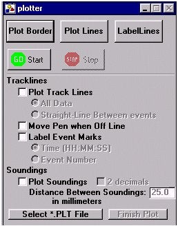
Figure 2: Plotter control window
最後に、Setupボタンをクリックします。ここで、プロッタ起点を選択します。シート左下のコーナー、または、センターを選択し、OKボタンをクリックし、Device Setupを終了します。再度OKボタンをクリックし、Hardwareプログラムを終了します。以上でSurveyにてプロッタを使用することが可能となります。
Surveyプログラムを起動するとプロッタをコントロールするダイアログボックスが表示されます。
Select *.PLT Fileボタンをクリックし、プロッティングシートを選択します。
境界線、計画測線をプロットする場合はウィンドウ上部のボタンをクリックします。
航跡を出力する場合、Plot Track Linesの隣のボックスをチェックします。これによって、航跡全てを出力するかイベントの間を直線で結ぶかの選択が可能となります。Move Pen when Off Line をチェックするとデータ収録を行っていない間(プロッタのペンが浮いている状態)でもプロッタのペンが航跡を追いつづけるようになります。
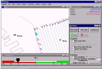
Figure 3: Plotter window in the Survey program
航跡上のイベントマークにラベルをつけることも可能です。ラベルは時間またはイベント番号のいずれかを選択できます。 測深値は、Plot Soundingsボックスをチェックすることによってリアルタイムプロットが可能になります。これにより、小数点2桁の出力、測深ポイント間距離の変化の出力設定が可能になります。
QTINモデルプログラムにおけるシングルビームデータの処理方法の改善(TIN Model and Single Beam Data)[英語]
There are many obstacles to create a useful TIN from a single beam data set. Although the data set might have a high level of accuracy the corresponding TIN can be almost unusable.
The main problem is to prevent the creation of undesirable triangles along the edges and wide triangles inside of TIN body. These triangles contribute to volume calculation error and contour accuracy.
To prevent such situations, we use the original planned line file that guided the vessel as the data was collected. The line file will prevent the TIN generator from connecting any three points that belong to the same line.
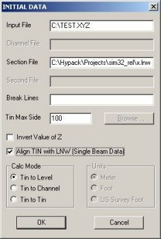
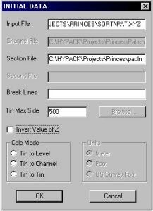
The Initial Data dialog has an additional check box that allows you to align the TIN and the corresponding line file. The line file name should be entered in the "Section File" field. Set the TIN Max Side as usual and click OK to create your model.
There are a few requirements regarding the planned line file:
- It can not contain intersecting lines.
- It can not contain a line without corresponding data.
- It must keep the lines in consecutive order.
Failure to meet any of the requirements will result in a badly created TIN that will lead to incorrect volume calculations and very strange contours.
An attempt to TIN multibeam data with the method will produce the same effect. The following pictures show the standard and the new methods applied to a real data set.
Looking at the first pair of pictures, you will see that we have achieved both goals:
- Eliminate wild triangles along the edges.
- Eliminate wide triangles inside the TIN body.
The second pair shows the contours. You can see that the new method eliminates all disruption along the edges or survey lines caused by poor triangle formation
The next set of pictures is an artificial example. Our first picture shows an imaginary channel 200m wide, 50m deep with 1:1 slope on both ends.
Four survey lines cross the channel at an angle of less than 45 degrees. The following pair of pictures are Solid TIN models with contours. You can see that the standard method creates bumps along the channel edge making a nonexistant volume buildup that affects the volume calculation. The new method calculates the volume (below 0.0 level) correctly 1 125 000.00 volume units. An error of about 1.3%.
Qイーサネットを利用したGPSデータの取り込み(Network monitoring of vessel position using NetNMEA driver)[英語]
The latest addition to the list of device drivers is the NetNMEA driver. This is a network ready driver that uses the UDP protocol to receive NMEA messages in a network environment. In conjunction with the NetNMEA driver a change has been made to the NMEA Output program in HYPACK Max to allow the NMEA Output program to send the NMEA messages to a UDP port. The following instructions explain the method used to configure both the sending and receiving of NMEA messages over the network.
Before we begin the actual steps of installing the device and configuring the port a little background information about IP addresses and Ports. Every computer on a network has an IP address. This is a series of 4 numbers that are individual to the computer. These numbers can either be assigned by a server dynamically or specified in the computer statically. In this explanation the IP addresses are going to be static. Most applications of the NetNMEA driver are going to be with static IP addresses. No two computers can have the same IP address or the computers would not know when to respond to a request. A typical IP address would be 192.168.1.2. This is the address of the Server at Coastal Oceanographics Inc. To see another computer on the network the computers must have IP addresses on the same sub-net. This brings us to the other half of an IP address. The Sub-Net. A sub-net is another series of 4 numbers that help define the network. In this application for the computers to see each other the sub-net must be the same. Now a bit about ports. Every computer has certain ports set aside for particular functions. Port 21 for example is the standard FTP port of the computer. Port 80 is the port used to access Web Pages on the computer. Ports are similar to windows. To hear what the neighbor is telling you, you have to be at the right window. Generally pick a port that is not used by the computer for something else. I used port 6650.
Now that the boring network stuff is done we can begin the actual setup of the computer to use this. To add the NetNMEA driver to the Hardware configuration start Hardware as you normally would and select Devices -> Add Device. The NetNMEA is listed in the device listing as NMEA-UDP just below NMEA-0183. Add this device to your setup. The configuration of the NetNMEA is similar to the NMEA driver.
The options for the NetNEMA driver are the same. I have chosen just position, speed and heading here. If I were setting this up to monitor another vessel the Echosounder option would most likely be checked as the NMEA Output program can convert the depth from the other vessel into a NMEA depth string independent of the type of Echosounder that is actually used.
The biggest difference between the NetNMEA driver and the standard NMEA driver is the Connect option. The NetNMEA driver uses the Connect to: Network option. Select the Change settings button to specify the port. The Hardware program was originally designed to have an IP address, Port and Computer Name for the remote computer. The only item that is required is the Port.
Remember from the boring network section that a port must be chosen to allow the data a window to pass through to us. This is all that is required to receive NMEA over the network.
To configure the NMEA Output program Select the Connect option and Choose network. It is critical that the sender, NMEA Output program know who is being sent the message. The NMEA Output program requires an IP address to send the message to. This doesn’t mean that if you don’t know the address of the receiving computer that you cannot send messages. Lets look at an example.
There are two dredges that are running in a Construction project. They are connected via a high speed wireless network. The dredge company decides to show both vessels on the screen in both dredges. This is our sample project. ( Yes, this is being done.)
Both dredges have GPS, Gyro and Depth. To configure the dredge with the ability to see the other dredge the NetNMEA driver must be added to the Hardware configuration of both dredges. The port must be different for each pair of connectors. Dredge 1 NetNMEA receives data from Dredge 2 NMEA Output program. They should have the same port specified as should the other pair. This device is added to another mobile in the hardware configuration. When the Survey program is run the user must start the NMEA Output program in Survey under Options -> Shared Memory so that data is sent to the other dredge. Once the program is running and the appropriate messages are selected the user starts sending data and the other dredge should be able to see the mobile on screen. If depth is desired for the other dredge send the DBT message and configure the receiving dredge with that message.
Just a quick note about sending messages. If it is desired to send the data to more than one other computer the message can be broadcast. This is also useful if the IP address of the target computer is unknown. In the NMEA Output program send the data to the IP address on the network ending in 255. In Coastal we would send the data to 192.168.1.255. This broadcasts the message.
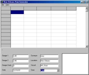
Qデジタイザで取込んだデータの使用(Shore Manual)
ショアマニュアルプログラム(SHORE MANUAL program)は、海岸線および海図記号を、Digitized Shoreline Format(*.DIG)へ手入力にて作成するために使用されます。これらのファイルはEDITINGとSURVEYプログラムにおいて表示されて、HYPLOTプログラムのスムーズシートにおいてプロットする事が可能です。
Shore Manual Dialog
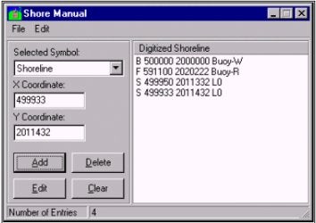
1..DIG Fileの作成法
- Selected Symbol項目のドロップダウンボックスからオブジェクト(Shoreline, Rock, Wreck, Buoy, 他)のタイプを選んでください。
- 選択したオブジェクトのX-Y座標を入力します。
- [ADD]ボタンをクリックします。選択した項目は、ウインドウの右側にあるリストに表示されます。
- 表示したいポイント数分ステップ1-3を繰り返します。
- FILE-SAVEまたはFILE SAVE ASをクリックし、ファイルを保存してください。デフォルトであなたのプロジェクトディレクトリに保存されますが、SAVE ASを使用すると、他の場所に保存することができます。
2. リストの編集
- 入力済みの変更したいポイントを選択します。そのポイントの情報は左側に表示されます。
- ポイントの情報を入力します。
- [EDIT]ボタンをクリックします。新しいデータが元のデータに置き換わります。
注意:もし最初から入力し直したいのであれば、[CLEAR]ボタンをクリックします。そうすると右のリストは全て消去されます。 - ファイルを保存します。FILE-SAVEをクリックし、.DIG拡張子を使用してファイルに名前を付けてください。ファイルはプロジェクトファイルに保存されます。
QSurveyプログラムの各種表示方法の設定について(Survey Schemes and the The New Schemebuilder Program)[英語]
What is a Scheme
In the newest version of HYPACK® Max, 02.6, coming out soon, Coastal Oceanographics, Inc. has developed the concept of "schemes" for the Survey program. Using schemes the HYPACK® Survey user has the ability to set color and font preferences for most of the screen objects in the Survey program, including the user interface colors for Windows®. The idea of schemes came about with the request of better day/night colors. Rather than setting colors we think the user might prefer for the night colors, schemes give the user the ability to set, and save, as many different color combinations as they prefer. Below is a screenshot of the Schemebuilder program.
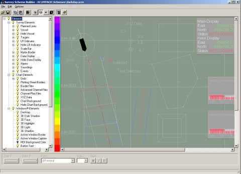
Image 1 - Schemebuilder program.
Using Schemebuilder
Launch Schemebuilder by clicking on the Settings->Schemebuilder menu item in HYPACK® Max. Using the program is very straight-forward. On the left you will notice a group of three different types of elements listed: Survey Elements, Chart Elements, and Windows® Elements. Survey elements are objects inside the program itself like the vessel colors, alarms, scale bar, etc. Chart elements are chart data types being drawn by Max's shared drawing engine. Windows elements are the colors of the user interface to your Windows® system (windows, desktop, etc.). When you click on one of the sub-items in the group its current color and/or font will be specified in the area below the window. You change the colors and/or font by selecting the new choice from a color/font dialog.
When you have specified the colors you would like for that scheme, you can then save the scheme into a .scm file. There a new directory under the HYPACK® Max root directory called 'Schemes' where the program will automatically attempt to save/open schemes from.
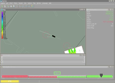
Image 2 - Survey program with the above scheme loaded.
Bring the Scheme into Survey
When running the Survey program, you can load a scheme by selecting the Options->Color Scheme... menu items. An open file dialog will appear with the directory set to the Schemes directory. Choose the scheme you prefer and it will become the default, meaning that it will load every time you run Survey thereafter (until otherwise specified).
QGeoTiFファイルを作成するユーティリティー(Freeware Program for Geo-referencing TIF Files)
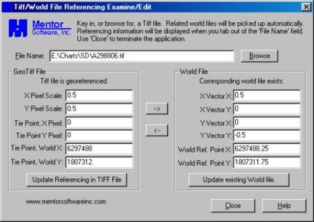
HypackではバックグランドデータとしてGeoTiffファイルの読み込みが可能となっています。この機能によ り航空写真などの画像ファイルを海図のように使用することが可能になります。GeoTiffファイルはTiffフォーマットのファイルに座標関連付けをす るTFWファイルを画像ファイルと同じフォルダに保存することで利用可能となります。
TFWファイルの内容は以下のようになっています。
- Xスケール (1ピクセルと実距離の比)
- Hypackでは未使用のフィールド
- Yスケール (1ピクセルと実距離の比)
- X基準座標
- Y基準座標
------------------実例---------------
1.50000000000000
0.00000000000000
0.00000000000000
-1.50000000000000
1934001.50000000000000
1187698.50000000000000
--------------------------------------
上例は画像ファイルのサイズが2000 X 2000、“x”基準座標が1934001.5でXスケールが1.5なので終点座標は基準座標から2000 * 1.5を加算した1937001.5となります。“y”基準座標は1187698.5なので 終点座標は2000 * -1.5を加算した1184698.5となります。
尚、GeoTiffファイルを作成するフリーウェアユーティリティプログラムが以下のWebサイトからダウンロードできます。
Mentor Software (http://www.mentorsoftwareinc.com) →サイトが閉鎖されました。
QUSB-シリアルポート変換機について(USB to Serial Devices: Just Say No!!!)[英語]
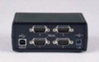
I've been beating this drum for about 2 years now. One of the most common hardware problems that we hear about is that the USB-to-serial devices always seem to be doing something screwy. We've seen everything from latency issues to flat out not being recognized by the operating system.
These devices, at one time, seemed very promising indeed. The truth about these devices has manifested itself over the last few years. The problem is that the "serial ports" they create are NOT real serial ports. They are considered "virtual" serial ports requiring the use of proprietary drivers that are not the standard Windows(R) communication drivers which Hypack(R) naturally prefers.
Other unadvertised limitations include:
Power loss over extended distances. (Any USB cable over 20 feet will seem to malfunction.)
If you use a USB port hub, it appears there is a power dilution effect that is directly proportional to the number of outlets in the hub.
High traffic sensors such as multibeam units, as well as heave, pitch and roll sensors, seem particularly susceptible to transmitting bad data. The advertised data rate does not reflect reality. I even had one unnamed company tell me that their device was not even compatible with GPS.
To be fair, some users have had success with USB to serial ports. All I can say about that is “wow” and “congratulations”. This may work for some very simple applications like one GPS and one echosounder. But if you ever come up with some funky data, don’t say that I didn’t warn you. Hypack®/Dredgepack®/Hysweep® cannot make a silk purse out of a sow’s ear. Bad data in, bad data out. The units made by Comtrol seem to have been the most successful. They have a network-to-serial device that seems to do trick much better. The bottom line is we just do not recommend them! We like the PCMCIA /PC Cards made by SOCKET I/O they have a ruggedized adaptor that precludes the use of duct tape to keep everything intact.
As of last year a “new” universal protocol for USB was adopted. USB 2.0. This promises to correct the data transfer “speed” of the previous incarnations of USB (1.0 and 1.1). The new data rate is supposedly equivalent to firewire. We shall see. The trick here is that you may buy a new computer with a USB 2.0 port but, if your USB-to-seria device is only USB 1.1 compliant, then you will gain no benefit from the new 2.0 protocol. In other words, you need both the computer and USB device to be the USB 2.0 code compliant. It remains to be seen if this will be acceptable for hydrographic surveying, as I have not seen any USB to Serial products for USB 2.0 yet.
Q新しいデバイスドライバ(New Device Driver for Dredgepack®)[英語]
The latest device driver for Dredgepack® was developed due to the need for a device that can be used to reference a position relative to a boat origin. This sounds confusing but it really is quite simple. In dredging terms the new device allows you to reference the position of the spud. By setting in the offsets from the boat reference point you can create a separate mobile that will give you position and distance from the center line of the spud. This is a critical piece of information when positioning a cutter suction dredge on a planned cut. By creating a center line the dredge operator can then use the spud XTE to ensure that the dredge is positioned properly.
Image 1
In Image 1 I have used the device to position 4 spuds, a crane pad and a working trailer on a barge. As the barge moves and rotates the objects onboard remain positioned properly. This should allow the user to create complex shapes to be displayed for easy reference.
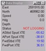
Image 2
The nice advantage of this new device is that the XTE can be displayed in the data display. On the shape I have a large dark blue square positioned where the crane pad is located. I have also added a smaller dark blue rectangle to show the location of the operators trailer. The four small light blue squares are positioned where the four spud holes are located.
In Image 2 I have captured the data display showing the reference to the four XTE values. This can be done for the X and Y of the spud also to allow exact positioning of an object for other applications such as position monitoring of a barge once it has been anchored. I believe that this new device driver will be very useful in the future applications of Dredgepack®. If you have specific questions regarding this device please e-mail me at jerry@coastalo.com.
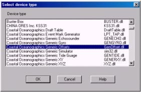
Image 3
Configuration of the GenOffsets driver.
The GenOffsets driver is a HYPACK® / Dredgepack® MAX device. This driver is used to reference a position as described in the previous document. The following description should allow you to add this driver to your hardware and use the device.
In the Hardware program you should select the Devices menu item and Add a Device. The Select Device Type window (Image3) will appear. In the list of devices you will then select Coastal Oceanographics Generic Offsets driver. This will load the device.
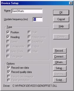
Image 4
The next screen (Image 4) is the device setup. The only options for this device are Position and Heading. The Heading box must be checked to allow the device to steal its heading from the main vessel. If you notice that the second shape does not rotate exactly with your main shape but lags a small amount this box is most likely not checked. I recommend setting the Update Frequency to the same rate as the positioning device. In the Record menu I recommend selecting the record option to never unless you are interested in recording the position of the device. For a spud you might want to set the record option to a predetermined number of seconds. This configuration will allow you plot out the location of the spud as it traveled through the cut. Also this will allow the plot to show the swing in relation to the spud position.
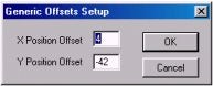
Image 5
Under the Setup option the button there is a X Position Offset and a Y Position Offset (Image 5). These offsets are used to locate the new item in relation to the reference point of the main vessel shape. The position referred to during this step is corresponding to the reference point of the shape you have created for your spud or other object.
The other important item to be completed in the Hardware program is to add this item as a Other Mobile. On the far right menu of the Hardware program is a option for the Other Mobile. To explain, the Other Mobile idea. A Other Mobile is a separate vessel displayed on the Map in the Survey / Dredgepack® program. This also allows you to display the parameters of the other mobile. Such as the X and Y of the mobile. Below is an image of the Hardware program.
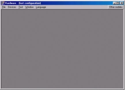
Harware Program
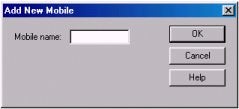
Once you have selected the Other Mobile the next option to choose is Add. This brings up the following menu. Name the new mobile and then select Ok.
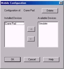
The next thing we want to do is to add our devices to the mobile. The image to the right is the Mobile Configuration menu. To reach this menu you need to select the Other Mobile button and then select the mobile name you entered. Using this menu you can add the devices to your mobile. This can include any device types that you would be using on the main vessel. In our application this is going to be the device we setup previously. I named my device Crane Pad. This refers to the location of the Crane Pad on the barge. To add a device to a mobile you first select the device in the box on the right labeled Available Devices. Once you have selected the device you select the arrow button sending the device to the list on the left labeled Installed Devices. This moves the available device to the mobile. All of the devices listed are then associated with the new mobile. If there is an echo sounder or other device the position is calculated using the position of the mobile and the offsets associated with the hardware.
In the Survey program you will now see two shapes. Using the new device you should right click on the main vessel and de-select the display shape. Once this is accomplished you can then right click on the second shape to select shape. Select the shape you would like to display. Once you have the new shape on the screen you should right click on the main vessel and select display shape. This will redraw your main vessel. As I showed in the original document there are many uses for such a driver. I hope that you have as much success with this driver as I have had.
QRTK GPSの特別な使用方法(Do Not Fudge RTK GPS)[英語]
A few years ago, in Hypack conferences, we were discussing about "fudged" differential systems. What is a "fudged" system? To get rid of the annoying and possibly inaccurate datum transformation, you enter local datum coordinates in the base station of a differential GPS system and you expect the rover GPS to output coordinates directly in the local datum. All GPS experts consulted at the time seemed to agree that such a technique is usable in a fairly large radius around the base station (over 100km if I remember correctly).
At the time it was a very useful technique for many of our users as datum transformation parameters were not readily available and Hypack didn't provide any support for finding even approximated parameters. Times have changed and now a user within continental US can calculate those parameters directly in the "Geodetic Parameters" program (using the CORPSCON button) and the rest can try to find an approximated value using the "Datum Transformation" program so the "fudged" systems have become somewhat obsolete.
Recently however I've seen someone trying to use a "fudged" RTK system and not with very good results: the rover GPS would drop out of RTK mode and it not come back even at very short distance from the base station. To see if it is safe to use "fudged" RTK systems let us examine closer how an RTK system works.
An RTK system achieves its incredible accuracy by measuring the "carrier phase" - this is the phase of the 1.52 GHz signal sent by satellites. The wavelength of this signal is approximately 19cm and its phase can be measured with a precision of about 1%. The only problem is that this signal repeats itself, well every 19 cm, so to find out your position the GPS receiver needs to calculate the number of integer cycles of 19 cm that fit along the path between itself and the satellite. This process is called "solving the integer ambiguities" and it is not an easy job (if it would have been, RTK receivers would have been available long ago and they would be much cheaper). Help comes from different sources:
- The pseudorange solution (the classical way of calculating a GPS position) gives an approximate position of the receiver thus narrowing the range of integer cycles that yield a possible solution.
- Knowledge about satellite's movement - a nice smooth ellipse - also helps if we are to sit longer in the same position (roughly speaking, if the receiver picks the wrong solution, the satellite doesn't follow it's predicted path so the receiver tries a different solution).
Assuming a receiver has found a good solution (the RTK loop is locked in GPS lingo) it still needs to differentiate between it's own movement and the satellite's movement and this is where the RTK base station comes into play: it transmits it's own carrier phase measurements so that the roving receiver can figure out how much of the change is due to it's own movement and how much is due to satellite movement. This is one of the main differences between differential and RTK GPS: the classic differential solution is a "discrete" solution that is calculated completely at every cycle with little information about the previous state of the receiver, while RTK solution is a "continuous" one in which information about the previous position is built into every new one.
What happens now when you "fudge" the system by entering coordinates in another datum than WGS-84? All of a sudden satellites don't follow their predicted path so your GPS receiver is going to be confused. More often than not it will not be able to properly solve the integer ambiguities and it will drop to a standard differential solution.
So our recommendation based on the little knowledge and experience we have with GPS systems is DO NOT TRY TO FUDGE AN RTK SYSTEM! Go out and find the correct datum transformation parameters, set your base station to correct WGS-84 coordinates and Hypack will obligingly calculate correct coordinates on your local datum.
I tried to get more information and opinions by posting this question on USENET discussion groups. Initial reactions seem to validate our opinion. If we are at it, you should try to visit sci.geo.satellite-nav and sci.engr.surveying. There you will find a wealth of information about GPS and surveying as well as informed people willing to answer your questions.
Qローカルグリッドの例(Local Grid--An Example)
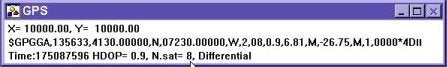
GEODETIC PARAMETERSのLocal GridオプションはGPSを用いた局地的なグリッドを使用することを可能とします。Hypack Maxは緯度/経度情報を得た後、それを指定した投影法(State Plane 1983,UTM等)のX,Y座標に置き換えます。それから、投影座標からユーザーがGEODTIC PARAMETORSプログラムのLocal Gridで指定した局地座標に変換します。
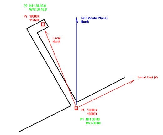
この例はどのように変換されているのかを表したイラストです。上図ではユーザは2つのポイントP1,P2を指定しています。このローカルグリッドでの座標は以下の通りです。
| P1 | X = 10000.0 | P2 | X = 10000.0 |
|---|---|---|---|
| Y = 10000.0 | Y = 11260.0 |
これらのポイントをWGS-84の緯度経度で表すと以下の様になります。
| P1 | N41 – 30 – 00.0000 | P2 | N41 – 30 – 10.0000 |
|---|---|---|---|
| W72 – 30 – 00.0000 | W72 – 30 – 10.0000 |
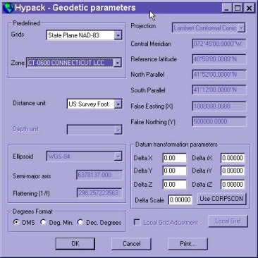
コースタル社はコネチカットにあるため投影方式はNAD-1983 CT State Plane Zoneを使用しています。はじめに行うべきことはWGS-84で示されるP1,P2の緯度経度をState Plane座標に計算しなおします。
始めにGEODETIC PARAMETERSプログラムを起動し、以図の様にNAD-83 CT State Planeを指定してください。
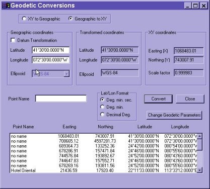
次に、GeodesyメニューからGRID COVERSIONプログラムを起動し、P1,P2をState Plane座標に変換してください。得られた結果は以下の様になるはずです。
| P1 | X = 1068483.01 | P2 | X = 1067719.20 |
|---|---|---|---|
| Y = 743007.91 | Y = 744017.87 |
P1とP2の間の距離とGridの北方向に対しての角度を求める必要があります。その結果は以下の様になります。
| Ang = 37.09939 degrees |
| Dist = 1266.26 |
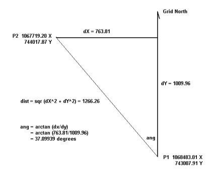
同じ計算を局地座標についても行います。P1,P2のX座標は同じであるため、局地座標での北方向の角度は0.0になります。また、Distanceは1260.0です。
ScaleはDistanceの縮尺率です。投影座標のDistanceが1266.6で局地座標のDistanceが1260.0の場合、縮尺率は0.9950565です。
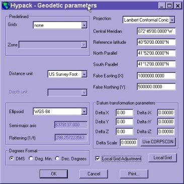
GEODETIC PARAMETERに戻り、残りのNAD-1983の設定を行います。GridsフレームをState Plane NAD 83からNoneに変更してください。これでLocal Grid Adjustmentのチェックボックスが有効になります。その時のウインドウの状態は左図のようになるはずです。
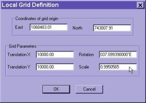
チェックボックスをONにし、Local Gridボタンをクリックしてください。局座標パラメータ入力ウインドウが現れます。P1を原点としてCT NAD-83 Stete Plane座標で準備してください。局座標で計算したP1のX,Yの値を入力してください。37.09939をRotationに、1.004968をScaleに入力してください。
パラメータを保存し、HARDWAREプログラムを起動し、GPSをP1の上に置き、Testプロセスを実行します。結果は下図の様に10000X,10000Yになるはずです。
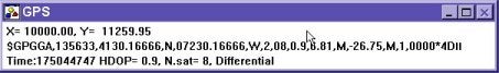
次にGPSをP2のポイントに置き同じテストを行うと、下図の様にX=10000,Y=12260を得るはずです。
Qインストールの仕方(An Ounce Of Prevention Is Worth A Pound Of Cure When It Comes To Installation)
HYPACK(TM)のインストールが、できるだけ簡単にできるよう、私達は努力してきました。CD-Rの普及に よって、インストールは大変簡単になりました。Coastal Oceanographics社でのインストールテストは、コンピュータをインストールに最適な環境にした上で行っています。その上で実感したことは、各 々のユーザーのコンピュータ環境と、私達のコンピュータ環境を全く同じようにすることができないという点です。その点に関しては、ユーザーの方々に少々の 手間を戴くことで、インストール不具合が起きにくくすることができます。

- HYPACK(TM)をアンインストールし、古いcoastalディレクトリを削除、または名前変更をしてください。
- CDを挿入する前に、現在実行中の全てのプログラムを終了させます。
Windows95/98では、ExplorerとSystray以外の全てのプログラムをCtrlキー、Altキー、Deleteキーを同時に押すことで終了させます。("シャットダウン"を選択しないでください) - 次にCDを挿入して、インストールを実行します。
7.1もしくは、それ以前のバージョンのHYPACKで使われていたiniファイルは使用しないでください。 - 新規にiniファイルを作成します。
シンプルで標準的な環境にする
もう一つ、やっておかなくてはならないことは、Autoexec.batとConfig.sysファイルから、不要な記述を無くすることです。Autoexec.batの中にある記述で、HYPACK(TM)コンピュータにとって必要なものは以下の行です:
SET PATH=C:\COASTAL
SET COASTAL=c:\coastal
コンピュータに十分詳しい人に、不必要な行をREMでコメントアウト、または削除してもらってください。
"スタート"メニューの"ファイル名を指定して実行"を選択して現れるダイアログで、"SYSEDIT"と打ち込んでください。WIN.INIに記述されているload と runの行は、値が入力されていないことにも気をつけてください。
また、スタートアップ項目(スタート-プログラム-スタートアップ)の中から、全ての項目を削除することを強く推奨します。
大概のメーカー製コンピュータには、多くのプリインストールソフトがインストールされていますが、これにより、オペレーティングシステムの調子が悪くなっ たり、インストールされているソフト同士での干渉が起こったりする危険性が生じます。HYPACK(TM)が、他のプログラムの不具合によって、影響を受 けないとは言えません。
コントロールパネルのアプリケーションの追加と削除で、使用しないソフトウェアを削除してください。最後に、マイクロソフトのウェブサイトhttp://www.slaughterhouse.com/へ行き、REGCLEANというフリーソフトをダウンロードしてください。このソフトにより、手動で取り除くことの難しい不要なレジストリエントリを削除することができます。
REGCLEANが見つからない場合は、東陽テクニカへ連絡下さい。
インストール時はスクリーンセーバーを全て解除しておいてください。スクリーンセーバーは、COMポートからの信号を検出しますが、COMポートに関する余計な処理は停止させなくてはなりません。
スキャンディスクやデフラグ(スタート-プログラム-アクセサリ-システムツール)を毎週行うことは、大変有効な手段でしょう。
つまり、HYPACK(TM)のインストールに望ましいコンピュータとは、以下のようなコンピュータであるということになります。
- メモリとリソースが最大限に確保されている。
- シンプルで標準的な環境にセットアップされている。
- 高速である。
- 不安定なプログラムによる干渉が極力無い。
QROVが操作エリアに存在するか確認する
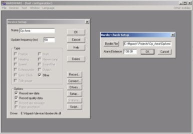
ROVのオペレーションのために新しいデバイスドライバを作成されました。ドライバの目的は、ROVがいつそのオペレーティング限界に達したかをオペレーターに通知することによってROVの安全なオペレーションを維持することです。
オペレータは、ドライバを利用するために、最初にHypackでBorderファイルを作成しなければなり ません。Borderファイルを作成しているとき、最後のポイントは、エリアの中または外で右クリックをします。この操作によって境界を閉じることができ ます。右クリックのロケーションは、ROVがその境界のどちらに存在するかによって決められます。あなたが境界の中でクリックするならば、ROVは、境界 内をオペレーションエリアとして扱います。そのドライバは、境界をオペレーションエリアとしても排他エリアとしても扱うことが出来ます。下記は、 Hardwareプログラムのセットアップの例です。
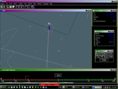
次のイメージは、Surveyプログラム上でバージニアビーチ沖のオペレーションエリアに入る軍艦を示しています。これは、港からオペレーションエリアの外へ出ることの計画トラックを用いて作成されたシミュレーションです。

上のイメージにおいて、船は、境界線の外にあり、アラームが表示されている。
このイメージにおいて、船は、100フィートのアラームリミット内に存在する。
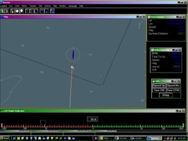
最終的に、船は、オペレーションエリアの内側にあり、オペレーションエリアの端への距離がData Displayにリストされることに注目してください。船の周りに、ビジュアルバッファアラームとして500フィートのサークルが表示されます。同じく船には、意図した動きのために10秒ベクトルが表示されます。
Q音線屈折処理について
レイトレーシング(音線追跡)は、マルチ‐ビーム水深測量の音線屈折を補正します。レイ・トレーシングの基本は音速度層を含むウォーターカラムを経た、音線のパスの十分な計算です。
SVプロファイル
音線計算は、音速度プロファイル(ウォーターカラムにおける各層の音速度の計測)で始まる。左下で示されたプロファイルは、河口において1.5フィート位毎で計測された典型例です。
第2のプロファイル(下記、右)においては、後続する計算を簡略化するために、おおよそ3ポイントにしています。
そのテーブルは、概略のプロファイルを与える。
|
層端の深度(Feet) |
層厚–h ( Feet ) |
音速度–V (Feet/s) |
|---|---|---|
|
10 |
10 |
4730 |
|
30 |
20 |
4775 |
|
50 |
無制限 |
4793 |
最終の層厚は無制限です。測定された深さがプロファイルの限界より大きい場合、無制限に底層が伸びるように、仮定されます。
深い水域において、圧力は、支配的要素となり、そして、音速度は、深さの関数として計算されます。
音線ダイアグラム:
音線ダイアグラムは、屈折のためのパス変更を含む音線のプロファイルビューです。それらの数値は、真の測深点に通じるレイ・トレーシングに必要とされる中間計算である。
V : 層の音速度。
Beam Angle q:鉛直に対する角度
Range r:各層の進行方向の距離
Depth d:各層の鉛直方向の距離
Offset s:各層の音線の水平位置
h : SV層高さ。
例において、水線(ドラフト)以下のソーナ深さは、4フィートです。屈折させられた音線は、グリーン、直線で結ばれた音線は赤で示されています。
上図は垂直-水平方向が1:1で描かれたものです。1つ明白なことは:深さは、レイ・トレーシングの対比とは異なって測定されていることです。
計算の前に非同種の弾力のある物質中の波の伝送を制御スネルの法則の基礎を理解することが必要です。:
sin(θ1) / V1 = sin(θ2) / V2 = sin(θn) / Vn = p
θ 鉛直方向に対する角度
V 音速度
p (一定の)音線パラメータである。
まず、ソナーによって供給された2つの測定を考察する; (1)スラントレンジr = 80.06フィート、及び、(2)初期ビーム角θ= 45度。(もちろん、ピッチ、ロール、マウンティングオフセットが加味されたものである)。
この例の場合、初期ビーム角45度、及び、表面音速度4730、音線パラメータp = 1.4949E-4を鳴らす。ダイアグラムにしめされた角度は簡単に計算できます。:
θn= p * Vn
θ1= p * V1= 45.00度。
θ2= p * V2= 45.55度。
θ3= p * V3= 45.77度。
次のステップは、各層を進行する傾斜距離rnを計算することです。:
rn = hn / cos(θn)
その式は、最初の2つの層で使用されます。第3の層は、我々は、トータルの傾斜範囲からの最初の2つの層で進行した距離を単に減じることで求められます。
r1 = h1 / cos(θ1)= 8.49 feet (h1 はドラフト6 feetが調整済み)
r2 = h2 / cos(θ2)= 28.56 feet
r3 = r – (r1 + r2) = 43.01 feet
測深値を計算するために、我々は、各層を進行する垂直方向の距離dを必要とします。最初の2つの層においてそれは、容易です。–単に層の高さとなります。第3の層では再び三角法に頼ることになります。:
dn = rn * cos(θn)
d3 = r3 * cos(θ3) = 30.00 feet
層の加算は、56.00フィート+ 4フィートドラフト修正=60.00フィートの補正されていない深さを導きます。
水平の距離sが各層において進行する様子も同時に必要とします。:
sn = rn * sin(θn)
s1 = r1 * sin(θ1) = 6.00 feet
s2 = r2 * sin(θ2) = 20.39 feet
s3 = r3 * sin(θ3) = 30.82 feet
加算によりトータルのオフセットs = 57.21フィートが導かれます。
いかにレイ・トレーシングが深さに、計算の相殺に影響をもたらすかを示すために、以下の表は、レイ・トレーシングを行った場合と行わない場合の比較を行っています。
|
|
深さ |
オフセット |
|---|---|---|
|
レイトレースあり |
60.00 |
57.21 |
|
レイトレースなし |
60.61 |
56.61 |
|
パーセント差異 |
1.0パーセント |
1.0パーセント |
最終的に、ソーナヘッドのXYポジション、及び、ボートの方向のデータが得られれば、最終測深ポイントXYZは、計算することが可能です。
結論:
2つの結果が得られます。:
(1)マルチ‐ビームを使用した測深ではレイトレースが必須であること。
(2)レイトレースの計算にはコンピュータが最適であるということ。
Qリアルタイムマッピング(Real Time Mapping of Multibeam Data in HYPACK®)
Surveyプログラムはリアルタイムで収録中のマルチビームソナーデータをマトリクスを使って水深毎に色分けしたマッピングを行なうことが可能です。マトリクス (*.mtx)は数百、数千の独立した長方形のセルから構成されます。Surveyプログラムはそれぞれのセル単位で水深値を保存し、色分けして画面に表 示することが出来ます。それぞれのセルはリアルタイムデータ収録中に測深済みの場所とその場所の水深値を色で知らせてくれます。マトリクスファイルは Designプログラムで作成することが出来、用途に合わせてセルサイズ、マトリクスサイズを変更できます。
Survey画面でマトリクスファイルを読み込むにはMatrixをクリック後、Loadをクリックしてください。 ファイル選択ボックスが表れ、読み込み可能なマトリクスファイルがリストとして表示されます。使用するマトリクスファイルを選択しO.K.をクリックして ください。
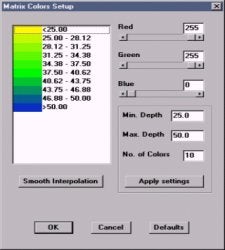
Figure 1: Matrix Settings dialog box in the Survey program
一度マトリクスを作成しSurvey画面にロードすると、Map画面の左端に水深毎のカラーバーが表示されます。カ ラーバーの水深、色を変更するときはカラーバーの上で右クリック後Settingメニューを選んでください。Settingでは始めに、最浅値、最深値、 色分けの数を指定します(図1参照)。Setting画面でApplyボタンをクリックするとSurvey画面にその色付けが採用されます。
色分けされたそれぞれのステップをクリックして、色をR-G-Bカラーバーから選ぶことが出来ます。色をスムージン グ(徐々にAからBへと色が変わる)をかけたいときは、その範囲内をドラッグし指定して、Smoothボタンをクリックしてください。処理終了後OK.ボ タンを押すと画面に結果が反映されます。
設定されたマトリクス範囲内での測量では、Surveyプログラムはマトリクスのセルに対して指定した色で塗りつぶしを行 います(図2参照)。各セルの水深データはマトリクスファイルに*.mtxのフォーマットで保存されます。MatrixメニューのSave as XYZからこれらの値をXYZのフォーマットで保存することが出来ます。ClearCurrentDataを選択することで現在表示されている色(水深 値)を全て消去することが出来ます。このコマンドを実行すると消去する前にデータを保存するかどうか 聞いてくるので、保存するときはYesしないときはNoを選んでください。UnloadメニューはSurveyプログラムから現在使用しているマトリクス ファイルを削除する場合に使用します。
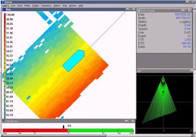
Figure2: Using a matrix to map multibeam data in Survey.
QEnd Area法体積計算の断面間の距離の決め方(Determining Distance Between Lines for Average End Area Volumes)
計画測線が平行である場合、測線間距離の決定はとても簡単です。計画測線が平行でない場合に問題が生じます。二本の測線間の距離決定は土量に影響を与えます。
例えば 、右図でArea1及びArea2(各々の計画測線上の面積)は、定数であり、計算結果の土量は、Lの値(測線間距離)が大きくなるにつれ増加します。
もし私が、港湾管理機関の人であれば、計算結果の土量を最少にするLの値を選び土量が少なくなるよう試みるでしょう。反対に、私が浚渫工事会社の人 であった場合、正しいLの値は出来るだけ大きな値に出来るものを主張するでしょう。双方の主張のバランスをとる為に、平行でない測線に対する、Lの値の決 定法が必要です。この章では我々が使用している所をみた、いくつかの方法について考察しHYPACK® MAX で使用されている方法について説明します。
Midpoint Method(中点法)
: 一つの方法は、測線の中点を結び測線間距離を決めます。右図の赤線がこの方法により決められた距離を示しています。
一方の測線がもう一方の測線にたいしてオフセットされていない状態の時には、この方法は良い近似を示す傾向があります。
右図にこの方法を使用しないであろう状態の例を示します。短い測線(Line1)と長い測線(Line2)が あるとします。各測線の中点は、測線に対して直行していません。この方法で計算されたLの値は二本の平行な測線の距離100’よりずいぶんと長くなってし まいます。これが結果として土量を多く見積もってしまいます。
Endpoint Method(端点法)
: その他の方法は、各測線の端点を結んだ線分を平均する方法です。右図では、Lの値を得る為にL1とL2を平均します。
この方法は、測線が同じ長さの時はかなりうまく機能します。うまくいかない場合は、下図に示すように一方が他方より長い時です。
この図で平行測線間の距離は100’です。しかし、Line1はLine2よりずっと短いです。この例では、 各端点間の距離は140’です。この値を使用するとこの部分で40%多く土量を計算してしまいます。このような場合、この方法を使用する事は不正と思われ てしまうでしょう。
Equal Area(等面積法)
: 最近我々がみた方法は線の両側の各面積を等しくするようにLの値を選択する方法です。
図で示すように、Lの値は、左側の面積(Area1)と右側の面積(Area2)が等しくなるように選択されています。
この方法は、おそらくその面積を通る線によって等しくされた面積”centroid”を決める為に開発されたのであろう。例の部分にて、この方法が一般にこの部分の土量を多く見積もってしまう事を示しましょう。
HYPACK® MAX Method(HYPACK® MAX法)
: 数年前多くのテストを経て我々は土量計算に使用する測線間距離決定の為のこの方法を提案しました。
Line1の中点を起点とし、Line2へ直行するように垂線をひきます。これをL1と呼びます。次にLine2の中点を起点とし同様に垂線を引きます。これをL2と呼びます。続いてLの値を決める為に、L1とL2の平均をとります。
この方法により、とても良い測線間距離の近似計算をほとんど全ての場合について行えます。
実例
: これらの方法を試し計算された土量の差を示す為に以下の例を示します。
Line1とLine2は左の点が接しています。Line1は100’の長さでLine2は116.62’の長さです。右端で60’離れています。これは右の三角形を形作ります。
入力した計画面より1’海底が上にあるとみなします。Line1上の面積は、100 ft² でLine2上の面積は116.62 ft²になります。
数学的に三角形の面積は3,000 ft²です。海底面が計画面より1’上にあるので数学的な土量は3,000 ft³です。
例: Midpoint Method(中点法)
: 各線分の中点を使用すると、L値は30’になります。これを平均断面法の公式にあてはめます。
V = L * (A1 + A2) / 2
V = 30. * (100. + 116.62) / 2.
V = 3,249.30 ft³ (+8.3%)
例: Endpoint Method(端点法)
: この方法を使用し、二本の計画測線、各々の端点間距離を計算します。左側の距離は0’であり右側の距離は60’です。従って平均の距離は30’です。この結果は中点法で使用した距離と同じになりました。
V = L * (A1 + A2) / 2
V = 30. * (100. + 116.62) / 2.
V = 3,249.30 ft³ (+8.3%)
例: Equal Area Method(等面積法)
: この方法では、Area1の面積(三角形)とArea2の面積(台形)が等しくなるようにLの値を計算しなければなりません。ちょっとした代数と幾何学を使いL値が42.43'であり、両面積は1,500 ft².になることが判明します。
この結果を平均断面法の公式にあてはめると下記答えがえられます。V = L * (A1 + A2) / 2
V = 42.43 * (100. + 116.62) / 2.
V = 4,595.59 ft³ (+53.2%)
例:HYPACK® MAX Method(HYPACK® MAX法)
: Line1の中点よりLine2へ垂線をひくと、その長さL1は25.72'です。Line2の中点よりLine1へ垂線をひくと、その長さL2は30'です。L1とL2の平均をとると、27.86’になります。
平均断面法の公式にあてはめると下記の答えがえられます。
V = L * (A1 + A2) / 2
V = 27.86 * (100. + 116.62) / 2.
V = 3,017.5 ft³ (+0.5%)
要約すると、HYPACK® MAX法によって計算されたL値が、数学的事実に最も近い平均断面土量となりました。これは、他の方法より我々の方法が優れていることを示す、我々が行ってきた数々の例中の単なる一例にすぎません。
QXYZファイルからマトリックス(MTX)ファイルを作成する(XYZ to MTX Program)[英語]
In our last newsletter, Lazar described a feature new to the TIN Model Program that converts the input XYZ data and outputs a filled, HYPACK® type Matrix file. The reaction from our users was so enthusiastic, we decided to make this feature a stand-alone utility. Here's how it works:
- Select PREPARATION-XYZ TO MTX and the dialog will appear.
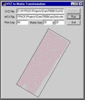
XYZ to MTX Transformation dialog
- Fill in all of the fields.
- Enter the XYZ file you wish to convert. ([Browse] makes it a snap!)
- Enter the path and name for your new Matrix file.
- Max Leg specifies the maximum distance used to connect to XYZ data points. This value must be greater than 0. Start with about 150% of your line spacing. You should set this large enough so your data points connect, but not so large that points which have little relationship connect to each other. The value of this field depends on the density of the input data. If the value is too small, the final result will be incomplete. If the value is too large, the creation will be slow.
- Matrix Size fields really define the cell size within the Matrix to be created.
- Click [Run]. The program generates a surface model and then calculates the Matrix size and rotation to fit the data. It then fills the matrix cells with the depth nearest the center of each cell calculated from the surface model.
A small representation of the results is drawn to the lower part of the dialog. You may also view the results by loading the Matrix file to the HYPACK® MAX screen.
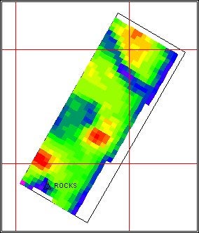
The resulting Matrix displayed in the main window
QHYPACKのSweepEditorプログラムで編集作業を行なっている時にサイドのデータが壁のように立っている。どうしてこのような事が起こるのでしょうか?測量時のプロセッサー画面にはそのようなデータは写っていなかったのですが...
マルチビーム計測の最中に、ソナーGUIのスワス画面(下の図)を見て下さい。
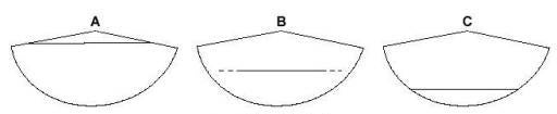
スワス表示位置
測量を行なっている時に、海底面がGUI上のイラスト「B」「C」のあたりに表示されていませんでしたか?
この部分に海底面が入っていると、円弧状より外のデータが取り扱われなくなってしまいます。イラスト「A」の部分(左右のデッパリより上)に海底面が入るようにRange設定を行なって、計測して下さい。