FAQ
FAQ検索結果
検索キーワード:
Qオンラインプロット機能(HYPACK 8.9 Online Plotting)
HYPACK 8.9測量プログラムのリアルタイムプロットの機能を使うために、適合の必要があるいくつかのハードウェアで考慮すべき事があります。
第一に、プロッター用ケーブルです。このケーブルは双方向通信をサポートしている必要があります。ケーブルには RTS-CTS の信号線が必要です。これらの信号線は、プロッターがプログラムに,いつプロッターが過負荷になっているかを知らせます。
これをすることによって、プロッターは、HYPACKから流れる情報量をコントロールすることができます。HYPACKの前のバージョンでは、そういった事例はありませんでした。
8.9へのアップグレードで、我々は、製図ルーチン用Windowsドライバーをもっと活用するためにこれを変えました。
次に考慮すべきことは、パラレルポートが双方向通信に対応しているかどうかです。 これは、ポートを介して情報を受け取れるかを示します。ほとんどのコンピュータは、この設定に問題がないでしょう。
プロッターの問題に直面したら、ケーブルをまず最初にチェックしてください。
それがRTS-CTSの信号線を持っているかを確認して下さい。
もしOKであれば、双方向通信をサポートするパラレル・ポート機能を持っていることを確認してください。
何かご不明の場合は当社にお問い合わせ下さい。
Qターミナルソフトを 使用して音速度のデータを収録しようとしているのですがセンサーからメッセージが帰って来ません。なぜでしょう?
電源供給にバッテリーを使用していませんか?
バッテリーを使用すると+12Vの端子に線を接続した時にセンサー内部ではリセット回路がONになったりOFFになったりしていて初期化がうまく行なえていない可能性があります。
バッテリーを使用せず、スイッチ付のAC/DC変換機をご利用下さい。
QGPSジャイロからヘディング(Heading)データが急に出力されなくなってしまいました。どうしたら良いでしょうか?
一時的に船外に設置されています3つのGPSアンテナの受信が遮られてしまった可能性が考えられます。
この時、本体内部ではヘディングデータの再計算が行なわれていますので次の様なデータ($PSER,ATTと$A)が出力されるまでお待ち下さい。(数分間お待ちください)
CS30E122A390S 5E 41A396S 6E 59A550S 8E 63A432S 9E 12A462S21E 47A 58S00E000A000S25E 68A203S00E000A000S29E114A23007D9
$PSER,ATT,064552.200,05,11,1998,+062.35,T,+01.63,-00.86,01.2,08>05,048,0
$A,0.1,+062.35,T,+01.62,-00.85,0
$A,0.2,+062.35,T,+01.62,-00.84,0
$A,0.3,+062.35,T,+01.61,-00.84,0
$A,0.4,+062.35,T,+01.61,-00.83,0
$A,0.5,+062.34,T,+01.60,-00.82,0
$GPGGA,064552.2,3526.336,N,13918.928,E,9,7,1,88,M,127,M
$GPVTG,299.3,T,,,0.02,N,,
$PSER,ATT,064552.800,05,11,1998,+062.34,T,+01.65,-
00.60,01.2,08>05,052,0
$A,0.1,+062.34,T,+01.64,-00.58,0
$A,0.2,+062.34,T,+01.64,-00.57,0
$A,0.3,+062.34,T,+01.63,-00.55,0
$A,0.4,+062.34,T,+01.63,-00.54,0
$A,0.5,+062.34,T,+01.62,-00.52,0
$GPGGA,064552.8,3526.336,N,13918.928,E,9,7,1,88,M,127,M
ヘディングデータの再計算中には、赤い部分のデータが出力されていません!
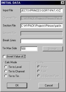
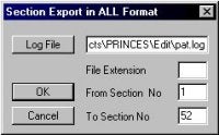
Q特定のエリアのXYZファイルを作成する(Clipping XYZ Survey Files to a Border File)
Clipping Survey Files
Borderファイルで規定された範囲に合わせて、ソートされたXYZファイルを抽出することができます。
- [Preparation-Editors-BorderEditor]を選択し、BORDER EDITORプログラムを起動します。
- [File-New]を選択し、新規ファイルの作成を設定します。
リストに多角形の頂点座標を加えるために、[Edit-Add point]をクリックします。
境界線が全て入力されるまでこの過程を繰り返します。このポイントにより、1つの連続したラインを形成し、最後の点は、このエリア内部の任意の点を入力します。
- [PREVIEW]をクリックすることにより、入力したイメージを確認できます。ポイントはスクリーンに表示されます(参照:プレビュー画面)。変更の必要がある場合は、BORDER EDITORを再び開き編集をする事ができます(参照:プレビュー画面)。編集する座標を選択し、[Edit-Edit point]をクリックし正しい座標値を入力します。

(図.プレビュー画面) - 入力後、[File-save]をクリックして、ボーダーファイル(*.brd)を保存します。
- Data File のSorted Data Files内のXYZデータを右クリックし[Clip to Border File]を選択します(参照:XYZデータの選択画面)。選択に使用するボーダーファイルの選択画面よりファイルを選択します。次に、選択されたXYZデータの名前を付ける画面が出るので名前を付け保存します。
(図.XYZデータの選択画面)
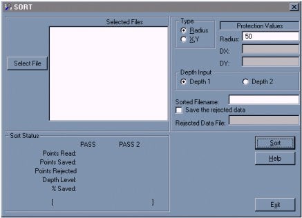
QHypackMaxデータ並替えプログラムのアップデート(Updated Sort Program in HYPACK® Max)
以前のバージョンのソートプログラムでは、ソートされるファイルはEditディレクトリからAvailableBoxに自動的に移動されていまし た。それからユーザが表示されているファイルを選択ファイルリストに加えてソートを行いました。この方法だと、ユーザのファイル選択に制限が加えられるこ とになります。
最新のソートプログラムでは、ユーザはどのプログラムでも選択してソートすることができます。ファイルをソートのリストに加えるのに2通りの方法がありま す。ソートダイアログボックスからSelectボタンをクリックするか、HYPACKプログラムからファイルをドラッグ&ドロップするかです。ユーザが Selectボタンをクリックすると、OpenFileダイアログボックスが現れ、ユーザは「*.log」「*.xyz」といったファイルタイプからファ イルを選ぶことができます。選択したファイルがSelectedFilesListの中に現れたら、OKをクリックしてください。
リストからソートを必要としないファイルを削除するには、ファイルを選択し右クリックしてください。ポップアップメニューから、ファイルを削除するかキャンセルするかを決定できます。
QDGN/DXFファイルからS57ファイルの作成(DGN/DXF to S57)
この機能は、DXFおよびDGNのファイルをインポートし、それらをS57形式のファイルに変える機能です。これ は、DXF/DGNファイル形式にふくまれるレイヤー情報を対応するDXF/DGNレイヤー上の形式に適合するS57形式のオブジェクトに指定する事によ り行われています。
この最初の変換が終了した後、個々のオブジェクトの属性をエディットすることができます。
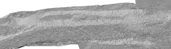
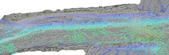
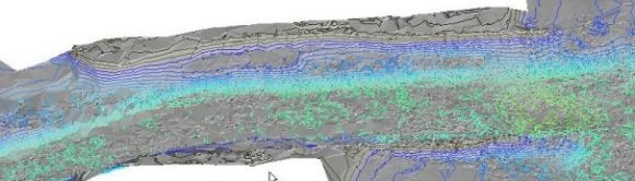
Q端側のデータが壁のように表示される
下の図を見て下さい。
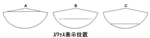
測量を行なっている時に、イラスト「B」「C」の部分に海底面が表示されていませんでしたか?この部分に海底面が、入っていると円弧状より外のデータが取り扱わられなくなってしまいます。
イラスト「A」の部分(左右のデッパリより上)に海底面が入るようにRange設定を行なって下さい。
Qエラーメッセージ(Incorrect or No Set Coastal Variable)
このエラーメッセージは、Coastal変数のあるディレクトリやフォルダを削除して しまった時、又はCoastal変数のあるディレクトリやフォルダのあるネットワークから接続を切断してしまった時に起こる共通のエラーです。ハードディ スクのディレクトリをもう一度作成するか、または、C:\coastal\datumディレクトリのWDATADIR.INIファイルを削除することで、 このエラーメッセージを回避することができます。
QRTK GPSによる潮位補正(Using RTK GPS in HYPACK for Real Time Water Levels)[英語]
Summary: Real Time Kinematic (RTK) GPS receivers can measure the latitude, longitude and height above the WGS-84 reference ellipsoid to within a few centimeters. Using this vertical accuracy, users can determine water level corrections (tide corrections). This eliminates the need to use conventional tide gauges or to assign personnel to monitor tide staffs. Users must establish their own RTK base station to supply differential corrections to the boat-GPS. In addition, users must pre-determine the separation between the WGS-84 reference ellipsoid and the appropriate chart datum in their survey area.
This paper provides a step-by-step explanation of using RTK GPS to obtain real time water levels in HYPACK(TM).
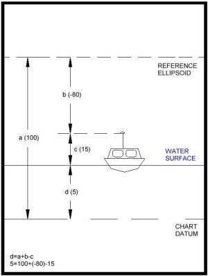
Figure 1: HYPACK(TM)'s method of obtaining real time water levels
Methodology
The figure to the right shows a survey boat using RTK GPS to determine the current water level correction.
Our measurements show the antenna height to be 15m above the static water line. This is the value (c) in the figure. c = 15.
The RTK GPS is reporting that the GPS antenna is 80m below the reference ellipsoid. This is value (b) in the figure. b = -80.
If we can determine how high the reference ellipsoid is above the chart datum [value (a)], we can then solve for the water level above the chart datum [value (d)].
In our example, we have pre-determined the reference ellipsoid is 100m above the chart datum. How we determined this is explained in the next section. From the diagram we can see that:
d = a + b - c
d= (100) + (-80) - 15 = 5m
Where (d) is the height of the water surface above the chart datum.
(a) is the height of the reference ellipsoid above the chart datum.
(b) is the height of the GPS antenna above the reference ellipsoid. This is supplied by your GPS.
(c) is the height of your GPS antenna above the static water line.
When correctly configured, HYPACK(TM) computes this value at each RTK GPS update and saves the position and a tide correction to the raw data file. The sign of value (d) is negated by HYPACK(TM) to be consistent with our normal tide correction values.
When the RAW data file from the SURVEY program is read into the Multibeam editor, each sounding will have an RTK Tide correction, based on the method shown above.
Determining the Separation between the Reference Ellipsoid and the Chart Datum
Before you head out on the water to start your survey, you need to determine the separation between the WGS-84 reference ellipsoid and the local chart datum. If your survey is conducted in a small area, you may need only a single point. If your survey is conducted over a large area where the separation between the ellipsoid and chart datum changes, you will need several points to Amodel@ the difference.
The following steps should be taken at each location to determine the separation between the reference ellipsoid and the chart datum.
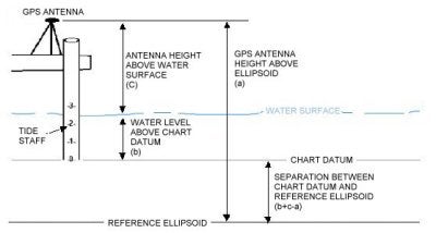
Figure 2: Determining the separation between the reference ellipsoid and the chart datum
Set up your GPS adjacent to your tide staff. The staff should be referenced to the local chart datum.
Write down the water level from the tide staff (b).
Measure the distance from your GPS antenna to the water level surface (c).
Once your GPS is stable and in RTK mode, write down the height of the GPS antenna above the reference ellipsoid. This is normally contained in the GGA and GGK messages. It might also be available on the front data display of some GPS. You should take care to note whether your GPS provides this value in feet or meters. If you are measuring depths in feet, you will need to convert the ellipsoid height of your antenna to feet. (1 meter = 3.280833333 feet). Record this value (a).
The height of the reference ellipsoid above the chart datum is equal to (b)+(c)-(a). In the diagram above, the reference ellipsoid is below the chart datum, so we would expect to get a negative number. The value will be a positive if the reference ellipsoid is above the chart datum and negative if the reference ellipsoid is below the chart datum.
Creating a KTD File
A Kinematic Tidal Datum (*.KTD) file is used in real time by the SURVEY program to determine the separation between the reference ellipsoid and the chart datum at the vessel location. This is used in cases where the separation between the two surfaces actually changes, depending on your location.
If the separation between your reference ellipsoid and chart datum is a constant, or if you are surveying in a small area and only want to use a single separation value, you do not need to make a KTD file. This is a new version of RTK Water Level implemented in HYPACK(TM) Version 8.1.a. and later. Details are presented in the next section.
To create a KTD file:
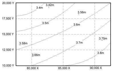
Figure 3: Separations: Ellipsoid above Chart Datum
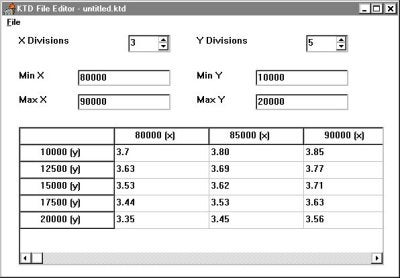
Figure 4: KTD File Editor
Plot your survey area on a piece of paper.
Plot the location of your tide stations, where you have determined the separation between the reference ellipsoid and the chart datum. Write the separation values next to each gauge.
Draw a rectangular grid around your survey area. This is the border of your KTD file. Make a note of the lower left X-Y and upper right X-Y coordinates. They will be needed when you create the KTD file.
Determine how many "nodes" you want in each direction. See the diagram to the right for an example. In this case, there are 3 nodes in the X-direction and 5-nodes in the Y-direction.
Contour the separation data, as shown in the figure to the right.
Determine a separation value at each node, based on the contour information.
Start the KTD File Editor. This program is only available in the 32-bit version of HYPACK(TM).
Enter the maximum and minimum values for your X and Y coordinates. These were obtained in step C.
Enter the number of nodes (or divisions) in each direction. The spreadsheet below will change to reflect the number you have entered.
Enter the separation value for each node in the appropriate grid.
When finished, click the File - Save and save the file to a KTD file. KTD files can be saved anywhere, but we normally put them in the \COASTAL directory.
In version 8.1 of HYPACK(TM) and earlier, users would enter a combined value that had the separation minus the static GPS antenna height. In Version 8.1.a. of HYPACK(TM) and later, you do not include the antenna height in the value entered in the KTD file. The TRIMKIN.DLL and KIN.DLL will obtain the antenna height from the offset information contained in the driver configuration.
Operating without a KTD File
As we mentioned before, a KTD file is only necessary if you are in an area where the separation between the reference ellipsoid and chart datum is not a constant. If the separation is a constant, or if your survey area is so small, you don't need more than a single value, you can operate without a KTD file.
You can "fool" the system by entering the combined value of your antenna height minus the height of the reference ellipsoid above the chart datum as the height in the "Offsets" window in HARDWARE for theTRIMKIN.DLL and KIN.DLL. This approach is only valid in HYPACK(TM) Version 8.1.a and later versions.
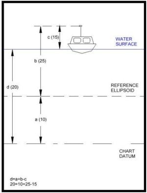
Figure 5: Operating without a KTD File.
For example, in the figure to the right, the antenna measures 15m above the static water line. The reference ellipsoid is 10m above the chart datum. We would enter 5.0 (15.0 - 10.0) as the antenna height and would not specify a KTD file.
While surveying, the SURVEY program receives a measurement from the RTK GPS, which shows the antenna is, located 25m above the reference ellipsoid. Since there is no KTD file, the program will assign zero to the separation value (a). Using our formula:
d = a + b - c
d = 0 + 25 - (5)
d = 20.
Using this technique, you don't have to mess with KTD files.
Setting up the Device Drivers to do RTK Real Time Water Levels
The KIN.DLL (Kinematic GPS) and TRIMKIN were written to provide real time water level capability in HYPACK(TM). You should configure them as you would any other GPS driver, with the following exceptions.
Make sure you have checked the "Tide" entry in the Type box. Otherwise, the driver will not perform the calculation to obtain a real time tide correction.
If you are using a KTD file, you need to select the KTD file in the Setup box.
・Make sure you specify the antenna height in the Offsets window. If you are using a KTD file, enter the height of the GPS antenna above the static water line. If you are working without a KTD file (see the section above), enter the height of the GPS antenna minus the height of the reference ellipsoid above the chart datum as your Antenna height.
Calibrating your Echosounder
In HYPACK(TM) version 8.1.a. and later, you should always calibrate your echosounder so the depth sent to the computer includes the measured depth from the transducer to the bottom, plus the transducer draft correction. In HYPACK(TM) version 8.1 and previous, you needed to have your echosounder output only the measured depth from the transducer face plate to the bottom.
Processing RTK GPS Data with Water Level Data
Provided you have correctly set up your survey to record real time water level corrections, processing is simple. The EDITOR program can read the raw format data file and use the TIDE records contained in the file automatically.
In the "Read Parameters" window, users can find the "Advanced" button. Clicking this button brings up access to the RTK Tide parameters. If the user clicks the RTK Tides check box, the EDITOR program will then use the RTK TIDE records written in the raw data file for tide corrections. This will activate the two options on how the program combines RTK water level elevations with heave corrections. The two choices will read:
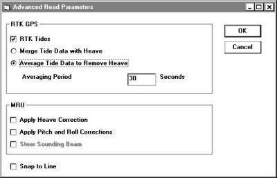
Figure 6: "Advanced Read Parameters" dialog box in the Editor program.
Merge Tide Data with Heave
Average Tide Data to Remove Heave
The "Merge Tide Data with Heave" uses the RTK elevations as vertical "anchors". Between the GPS elevation updates, the program "fits" the heave data to predict the change in vessel movement.
The Average Tide Data to Remove Heave averages the RTK elevations over a user defined time period to obtain a "normalized heave plane". In theory, this average vertical level should be the zero plane as defined by the heave-pitch-roll sensor. The program then applies the exact heave corrections to the data to obtain the exact vessel position at the time of the depth measurement. A time period of 30 seconds seems to work quite well.
Editing RTK GPS Data with Conventional Tides
Users can process raw data files that have RTK water level corrections using conventional tides by simply reading a TID file while in the EDITOR spreadsheet. This allows you to process the data using RTK water levels or conventional tide corrections and then compare the results in the CROSS SECTIONS program (or in the EDITOR profile screen by using the Overlay feature).
Q新しいXYZ出力ユーティリティー(Changes in XYZ Export in TIN MODEL)[英語]
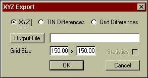
While I was down in Florida demonstrating the TIN MODEL to a client, I was surprised to see that the XYZ Export options in TIN MODEL had been expanded. Instead of being included in the Matrix Export window, the XYZ Export now has its own window, shown in the figure to the right.
It was a little confusing at first, but I quickly figured out the available options.
XYZ:
This is similar to the old XYZ Export option of the TIN MODEL. It is used to output a gridded ASCII XYZ file at user defined spacing. The user can enter the X and Y spacing (150 x 150 in our example above). The TIN MODEL program then takes the current surface model and determines the Z-value of the model at the grid’s nodes. It exports these values to the user-supplied name.
TIN Differences:
This was also available in the old TIN MODEL version. It is used to generate a model that represents the difference in z-level between two input models. A good example of its use would be in a beach erosion study, where you have two surveys done at different times of the year.
This routine takes the primary model (shown in red) and computes the level above (positive) or below (negative) a secondary model (shown in black). Each computed difference is then saved as the z-value for the x-y pair. The result is an ASCII XYZ Difference file that can then be read back into the TIN MODEL to show where material has accumulated or depleted. By calculating the volume of the differences above/below the 0 level, you can determine if you have had a net gain/loss of material during the study.
Grid Differences:
This is a new routine for the TIN MODEL. It is similar to the TIN Difference method, but instead of outputting the z-differences at the nodes of a model, it outputs the z-difference between two models at the user-specified spacing.
In the example shown to the right, the program would compute the z-difference (primary z-value minus secondary z-value) at a regular spacing, as defined in the XYZ Export window.
The resulting file can also be read back into the TIN MODEL to compute the net gain/loss of material between the two surveys.
All of these output files are in ASCII XYZ format and can be imported back into HYPACK® MAX or most other applications.
Q対応デバイス一覧
以下の表は現在HypackMAXで用意されているドライバです。下記表にない場合でも、NMEA.DLL のような
一般的なドライバを使用することで、多くのデバイスは動作することが可能です。
|
586xy.dll |
DelNorte 586 in XY mode |
|---|---|
|
adgc.dll |
KVH Digital Compass |
|
apl1a.dll |
Topcon apl1a |
|
ash3df.dll |
Ashtech 3DF GPS |
|
Atlanta.dll |
Laser Atlanta Range/Azimuth |
|
ats.dll |
Ats (Range-Azimuth) |
|
autop.dll |
NMEA Auto Pilot |
|
Bathy1500.dll |
Ocean Data Bathy 1500 |
|
Bathy500.dll |
Ocean Data Bathy 500 |
|
beep.dll |
Coastal Oceanographics Event Mark Sounder |
|
buster.dll |
Buster Box |
|
CableCnt.dll |
NOAA Cable Counter |
|
cap6000.dll |
Datasonics CAP-6000 Output |
|
CDLTilt.dll |
CDL mini tilt |
|
chkvh.dll |
CHKVH Gyro |
|
chsp20.dll |
Novatel RTK GPS (CHS) |
|
Chtide.dll |
Shanghai Tide System |
|
clinomet.dll |
clinometer driver |
|
clinoser.dll |
Generic Serial Bubbler/Clinometer |
|
ctd.dll |
Falmouth Scientific - Micro CTD |
|
cu3346.dll |
Aandera 3346 Tide Gauge |
|
ddr101a.dll |
DDR-101A Sounder |
|
Delph.dll |
NOAA Delph Output |
|
deso15.dll |
Atlas Deso 15 |
|
deso17.dll |
Atlas Deso 17 |
|
deso20.dll |
Atlas Deso 20 |
|
Deso20s.dll |
Atlas Deso 20s |
|
Deso20ss.dll |
Atlas Deso 20 serializer |
|
deso25.dll |
Atlas Deso 25 |
|
Dolphin.dll |
ROSS Dolphin (BCD) |
|
dovat75.dll |
Dova T75 Angle Sensor |
|
dpp1b.dll |
Navitronics Dpp1b serial echosounder |
|
DraftTable.dll |
Coastal Oceanographics Draft Table |
|
dsf6000.dll |
Ocean Data DSF-6000 (NOAA) |
|
dtrace.dll |
Odom Digitrace |
|
ea300.dll |
Simrad EA300 Echosounder |
|
ea500.dll |
Simrad EA500 echosounder |
|
echomod4.dll |
Odom Echotrac (NAVOCEANO Mod4) |
|
echoscan.dll |
Odom Echoscan (Multi-Transducer) |
|
echotrac.dll |
Odom Echotrac |
|
echoxl.dll |
Trimble Echo-XL Helmsman |
|
edgetech.dll |
USGS - Slant Range |
|
egg260.dll |
EG&G 260 magnetometer |
|
egg876.dll |
EG&G 876 Magnetometer |
|
egg880.dll |
EG&G 880 Magnetometer |
|
eggevnmea.dll |
Edgetech 260 |
|
eggnmea.dll |
EdgeTech Special NMEA Sentences (Output) |
|
Elac4300.dll |
Elac MKII Hydrostar 4300 |
|
elics.dll |
Delph Elics Side Scan (Output Only) |
|
elics1.dll |
Delph Elics side scan (output only) |
|
Entek.dll |
Entek SeeLevel Tide Gauge |
|
eod.dll |
Simrad (EOD) |
|
EPC.dll |
USGS - EPC Recorder |
|
EPCTape.dll |
EPCTape 1086 |
|
e-sea.dll |
Marimatech E-Sea Echo Sounder |
|
fahrenth.dll |
Fahrenth 32bit |
|
falcon.dll |
Motorola Falcon |
|
falcon4.dll |
Motorola Falcon IV Range/Range |
|
Fluoro.dll |
Fluorometer |
|
furuno.dll |
Furuno Video Plotter (Output Only) |
|
FurunoDPT.dll |
Furuno echosounder |
|
Gendevall.dll |
Coastal Oceanographics generic offsets |
|
genecho.dll |
Coastal Oceanographics Generic Echosounder |
|
generxy.dll |
Coastal Oceanographics Generic XY |
|
gengyro.dll |
Coastal Oceanographics Generic Gyro |
|
genoffset.dll |
Coastal Oceanographics generic offsets |
|
gentide.dll |
Coastal Oceanographics Generic Tide Guage |
|
geodats.dll |
geodemeter ats 600 (binary message) |
|
geodimet.dll |
Geodimeter (Range/Azimuth) |
|
geodmet2.dll |
geodimeter (range/azimuth) |
|
geog880.dll |
Geometrics G880 Magnetometer |
|
geog881.dll |
GeoMetrics Magnetometer |
|
geog881a.dll |
GeoMetrics 881 Magnetometer (Maryland modification) |
|
GyroTrac.dll |
GYRO_TRAC Device |
|
hhpr.dll |
Honeywell HPR |
|
hpgl.dll |
HPGL online plotter |
|
htg5000.dll |
Hazen HTG-5000 Tide Gauge |
|
hydro700.dll |
Odom Hydrotrac 700 Range/Range System |
|
hydroii.dll |
Laser Technologies Hydrolink II (USGS) |
|
hydroml.dll |
Laser Technologies Hydrolink (Modem Link) |
|
HySweep.dll |
Coastal Oceanographics HySweep Interface |
|
ihc.dll |
suction tube position monitor |
|
inn440s.dll |
Innerspace 440 (Serial) |
|
inn448.dll |
Innerspace 448 (Serial) |
|
inn449.dll |
Innerspace 449 (Serial) |
|
Isis.dll |
NOAA Isis |
|
Isiseod.dll |
Isis (Triton) EOD |
|
Isisout.dll |
USGS Isis output |
|
k320s.dll |
Knudsen 320M (CHS Serial) |
|
kin.dll |
NMEA Kinematic DGPS (Real Time Tides) |
|
kinematic.dll |
kinematic GPS (RTK tides) |
|
klein.dll |
Klein 595 & System 2000 Side Scan (Annotation/Speed Only) |
|
knu320ms.dll |
Knudsen 320M (Serial) |
|
kss31.dll |
CHINA ORES Inc. KSS31 |
|
kvh.dll |
Fluxgate Compass |
|
kvh_ad.dll |
KVH Azimuth Digital Compass |
|
laz4100.dll |
Allied Signal LAZ-4100 Echosounder |
|
lcd3.dll |
Coastal Oceanographics LCD3 Helmsman |
|
lcd4.dll |
Coastal Oceanographics LCD4 Helmsman |
|
Leica.dll |
Leica Total Station |
|
lineswitchin.dll |
line switch input |
|
lineswitchout.dll |
line switch output |
|
llq.dll |
Leica RTK GPS |
|
lpt_tap.dll |
Coastal Oceanographics Event Mark Generator |
|
lt_L5000.dll |
LaserTrack L5000 range/azimuth |
|
lt_L5001.dll |
LaserTrack L5001 range/azimuth |
|
Lundahl.dll |
Lundahl RST-1 air transducer |
|
mag7400.dll |
Magnavox MX7400 DGPS |
|
mandraft.dll |
USGS manual draft |
|
manual.dll |
Coastal Oceanographics manual entry |
|
mdtotco.dll |
MD Totco Series 2000 |
|
meconaut.dll |
Meconaut bubler system |
|
mkii.dll |
Odom MKII Echosounder |
|
mru6.dll |
Seatex MRU motion sensor |
|
MultiBCD.dll |
Ross Multi-Transducer (BCD) |
|
nm788.dll |
Motorola Miniranger III (NM788 Serial Interface) |
|
nmea.dll |
NMEA-0183 |
|
nmeakl.dll |
NMEA In, Klein Out |
|
nmeatkv.dll |
NMEA TKV Message (Speed/Temp) |
|
NoaaKnud.dll |
Knudsen 320 (NOAA) |
|
novax.dll |
Novatel PC card |
|
novoem.dll |
Novatel OEM Card |
|
novp20.dll |
Novatel RTK GPS |
|
Octopus460.dll |
Octopus 460 |
|
os200.dll |
OS200 |
|
osifloro.dll |
Turner Fluorometer |
|
otfgyro.dll |
Coastal Oceanographics OTF gyro/comparison |
|
outinfo.dll |
Coastal Oceanographics OutInfo |
|
pas900.dll |
Datasonic PAS-900 |
|
pdr130.dll |
Seabon PDR-130 Echosounder |
|
pdr6011.dll |
Seabon PDR-601 (Single Channel) |
|
pdr6014.dll |
Seabon PDR-601 (Four Channel) |
|
polar2.dll |
Polarfix Range/Azimuth (Beach Profile) |
|
polarfix.dll |
Polarfix Range/Azimuth |
|
polartrk.dll |
PolarTrack |
|
PosMV.dll |
TSS POS/MV |
|
printer.dll |
USGS - Printer |
|
ps20r.dll |
Kaijo PS-20R Echosounder |
|
ps30r.dll |
Kaijo PS-30R Echosounder |
|
qtc.dll |
Tangent'sQTC View Seabed Classification |
|
rhotheta.dll |
Del Norts Rho Theta (Range/Azimuth) |
|
rockser.dll |
Rockwell Collins 3A/DGPS (Serial) |
|
ross603.dll |
Ross 603 Echosounder (BCD) |
|
rossmart.dll |
Ross Smart Echosounder (Serial) |
|
roxann.dll |
Roxann Seabed Identification |
|
rtkcp.dll |
TRIMBLE RTK Cycle Printout |
|
sdig30.dll |
Navitronic Soundig 30 Echosounder |
|
Sdyne.dll |
Sonardyne USBL device |
|
seaspy.dll |
Marine Magnetics Seaspy magnetometer |
|
sercel.dll |
Sercel Axyle (XY mode) |
|
sgbrown.dll |
sgbrown gyro driver |
|
Shtube.dll |
Shanghai suction tube indicator |
|
sim32.dll |
Coastal Oceanographics generic simulator |
|
singlbcd.dll |
Ross Single-Transducer (BCD) |
|
sitex.dll |
Sitex Positioning System |
|
sixgun.dll |
Motorola Sixgun DGPS |
|
smartCTD.dll |
Smart CTD |
|
Smartswp.dll |
Ross SmartSweep |
|
smm_ii.dll |
Thomas Marconi SMM II Towed Magnetometer |
|
sms.dll |
Scandinavian Microsystems LR20,40,60 |
|
sonar_tm.dll |
Sonar Research & Development Tide Guage |
|
sonarlite.dll |
LM Technologies SonarLite device |
|
sound50.dll |
Navitron Sound50 echosounder |
|
sperry.dll |
Sperry Gyro |
|
star.dll |
Odom Star (Range/Azimuth) |
|
stpi.dll |
suction tube position indicator |
|
svp16.dll |
Applied Microsystems Sound Velocity Probe |
|
tds1000.dll |
TDS 1000 Echosounder |
|
testdev.dll |
Coastal Oceanographics Simulation |
|
Tidalite.dll |
Tidalite tide guage |
|
tidefile.dll |
Coastal Oceanographics Tides (From File) |
|
tjcut.dll |
TianJing cutter-suction |
|
trackp.dll |
Trackpoint II ROV Acoustic System |
|
trieod.dll |
Triton (EOD) |
|
trimcp.dll |
Trimble DGPS Cycle Printout Message |
|
tripmate.dll |
Tripmate GPS |
|
trisp.dll |
Del Norte Trisponder 542 |
|
trkplxt.dll |
Trackpoint LXT ROV Acoustic System |
|
tss320.dll |
TSS Motion Reference Unit |
|
Valeport.dll |
Valeport tide guage |
|
vynerlp.dll |
Vyner-LP Tide Gauge |
|
XYZ.dll |
Coastal Oceanographics Generic XYZ |
以下のリストはHysweepで使用される機器のドライバです
|
Atlas Bomasweep |
Multiple transducer driver |
|---|---|
|
Atlas Fansweep (Network) |
Multibeam driver--network interface |
|
Atlas Fansweep (Serial) |
Multibeam driver--COM port interface |
|
Hypack Max |
Link to Hypack Survey |
|
KVH Gyrotrac |
Heading, pitch and roll driver |
|
NMEA-0183 Gyro |
Gyro driver for NMEA HDT messages |
|
Odom Echoscan II |
Multibeam driver |
|
Odom Miniscan |
Multiple transducer driver |
|
Reson 8101 |
Multibeam driver |
|
Reson Seabat 9001 |
Multibeam driver |
|
Reson Seabat 9003 |
Multibeam driver |
|
Reson Sebat 81xx (Serial) |
8124, 8125 and newer 8101 multibeam driver--COM port interface |
|
Ross Smart Sweep |
Multitransducer |
|
Seabeam SB1185 |
Multibeam driver |
|
Seatex MRU6 |
Heave, pitch and roll driver |
|
SG Brown 1000S Gyro |
Gyro driver |
Q外部プログラム起動ユーティリティー(Launching External Programs from the Hypack® Max Menu)[英語]
You can use the EXTERNAL PROGRAMS menu that will launch external executable files. Just another handy alternative to using the usual Windows® methods.
- Select EXTERNAL PROGRAMS-SETUP. The Tool Options dialog will appear.
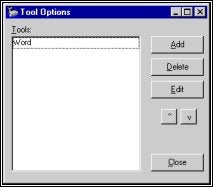
Tool Options dialog
- Click [Add] and the Tool Options Properties dialog will appear.
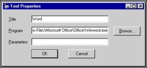
Tool Options Properties dialog
- Fill in the fields of the dialog then click [OK] and close the program.
The contents of the Title field will now appear in the Hypack® Max Help menu. In the future, when you select this menu item, it will launch the Program named in the second field and pass it any Parameters that you have listed.
The Current Project checkbox (not pictured here) is for internal use at Coastal Oceanographics Inc. only.
You can add as many programs as you want in this manner and use the up and down arrow buttons to arrange their order if desired.
To remove programs from the menu:
Open the Tool Options dialog, select the program to be removed and click [Delete].
To change the properties of any listed program:
Open the Tool Options dialog, select the program then click [Edit]. The Tool Options Properties dialog will appear with the current data and you can edit it as desired.
QADCPを利用する(ADCP Programs in Hypack Max)[英語]
ASB Systems, Coastal O's affiliate in Mumbai, India, has been hard at work on the development of our new ADCP data collection and processing modules, which will be included in the next release of HYPACK® Max. These modules have been designed to log data from RD Instruments' Workhorse ADCP's.
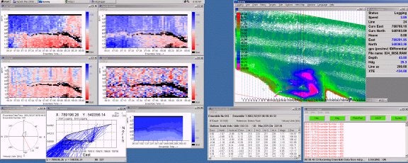
Figure 1: Hypack®’s ADCP Logger and Survey programs
The first module developed is the ADCP Logger. This module is designed to run alongside the HYPACK® Survey program, logging ADCP data simultaneously with HYPACK® raw data. The program uses RDI's ADCP configuration files to deploy the ADCP. The Logger has numerous display windows, including velocity profiles, intensity profiles, current magnitude, and tabular displays. The logged data files contain RDI raw data from the ADCP, in addition to navigation data passed from the Survey program through Shared Memory and into the Logger. The user also has the option to log standard RDI *r.000 files.
The next module is the ADCP Profile program. This program allows the user to load HYPACK's edited files and ADCP files, and get a cross sectional view of the survey line, echosounder depth or ADCP bottom track, and also display the current velocities. The user can then print or plot these profiles, and also calculate discharges and print a report.
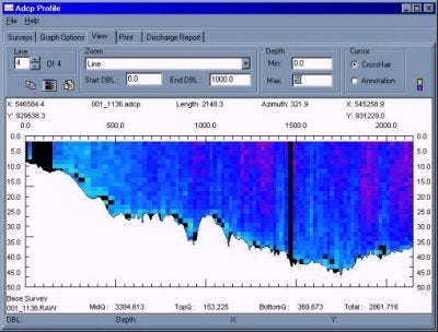
Figure 2: ADCP Profile program
Last but not least is the ADCP to DXF program. This program was created so that the user can create DXF current vectors from the data collected in Survey and the ADCP Logger. The user can specify vector length, vector type, current depth level and current speed units. These DXF vectors can then be imported into CAD/GIS packages, or plotted right in Hyplot®.
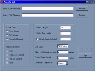
Figure 3: ADCP to DXF program
Q測深データ削減プログラム(Tests of Sounding Reduction Program)
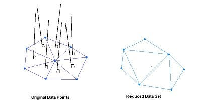
SOUNDING REDUCTIONプログラムはHYPACK(TM) Version 8.9のモジュールの一つとして製作・公開されたものでした。これは元データを忠実に反映しつつデータ量を減らした、サブセットを作り出すことを目的とし ています。例えば、1チャンネルのマルチビーム測量によって、5,000,000データ点数に昇ったとします。このデータをSOUNDING REDUCTIONプログラムに通すことによって、同じチャンネルを800,000データ点数で正確に描くことが可能です。
SOUNDING REDUCTIONでは、海底斜面の変化があるところでは、数多くのデータ点を保存します。比較的平坦な場所においてのみ、データ点を減らします。これは最近、LIDAR(airborne hydro)でのデータ簡略化や陸測データにおいて用いられた方法です。
このプログラムは、HYPACK(TM) SWPファイル(直接指定するかLOGファイルから指定するか)、アスキー形式のXYZファイルのどちらでも使用することができます。このプログラムに よって、右図に示されるように隣り合ったデータ点間で三角形を形成します。そして、各々の三角面から垂直に投影された線分の角度差を計算します。これらの 角度差がユーザーの指定した許容値以内であれば、中心点は"不要な"点として、データセットから外されます。角度差が許容値を超える場合には、その点は海 底面を正確に描くために必要な点として保存されます。
SOUNDING REDUCTIONプログラムの実行は簡単です。まず入力ファイルを開きます。アスキー形式のXYZファイルもしくは、HYPACK(TM) SWP ファイル(直接指定するかLOGファイルから指定するか)を選びます。データを読み取り、いくつの測深点が記録されているのかを表示します。
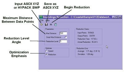
次に、除外するための角度と(マルチビームデータは10°を指定すると良いようです。)、データ点間の最大距離を入力します。この最大距離によっ て、平坦な場所において、代表点を保持することができます。入力が終わったら、計算を実行させます。データ点数によりますが、せいぜい数分で計算が終わり ます。最後に、この計算結果をアスキーXYZファイルへ保存します。
SOUNDING REDUCTIONプログラムをテストするに当たって、データファイルは、USACE-TECより提供されました。データ点数515,420を、異なる"除外角度"を用いて計算させました。結果は以下の表にまとめてあります。
|
削減設定角 |
実行時間 (secs) |
% 削減率 |
# 最終的なデータ数t |
|---|---|---|---|
|
Original Data Set |
515,420 |
||
|
5 |
116.72 (2 iterations) |
35.25 |
333,791 |
|
6 |
116.11 |
42.05 |
298,675 |
|
8 |
163.84 (3 iterations) |
54.14 |
236,388 |
|
10 |
158.52 |
61.94 |
196,144 |
|
12 |
152.69 |
68.11 |
164,375 |
|
14 |
147.04 |
73.03 |
139,014 |
|
16 |
141.27 |
77.06 |
118,237 |
|
18 |
135.56 |
80.40 |
101,008 |
|
20 |
129.79 |
83.20 |
86,609 |
|
25 |
143.41 (4 iterations) |
88.64 |
58,572 |
|
30 |
127.32 |
91.77 |
42,471 |
計算時間は除外角度によって異なっています。計算は、細部の繰り返しによって点の除外率が小さくなると自動的に終わります。
結果がもっとよくわかるように、以下にHYPACK(TM) TIN modelを用いて作成した三つの表面モデルを示します。
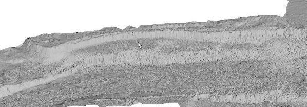
Original Data Set
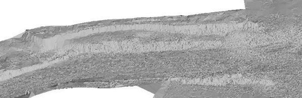
10 Degree Reduction (61.94%)
20 Degree Reduction (83.20%)
除外角10°を超えると表面モデルは劣化していますが、実際の等深線は、それほど悪くはありません。
Original Data Set with 3' Contours.
20 Degree Reduced Data Set with 3' Contours.
QDregepackとSurveyプログラムにおけるマトリックスオプション(Matrix Options in Dredgepack® and HYPACK® Max Survey)[英語]
New Options:
A couple of new options have recently been added to the Hypack® Survey and Dredgepack programs that may interest you. The one that is particularly interesting to me is found in the Matrix Options dialog in each program. In the past, the matrix data has been updated whether you were online or offline. Now you have the option to choose when data will be entered to the Matrix.
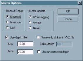
The Matrix Options Dialog
The Matrix Update option enables you to choose when soundings will be drawn to the matrix.
- While Logging paints the matrix only while you are online. This will enable the matrix data to coincide with the survey data.
- Always paints the matrix whether you are online or not (as before). This option enables you to follow your dredging in the Matrix while not recording the Raw data if you don't need it.
- Never tells the program not to update the matrix. You can display the matrix without changing the data.
The Use Uncorrected Depth is a new option requested by one of our users. Very simply, gives you the choice to store raw depths or corrected depths to your matrix.
Depth Mode vs. Elevation Mode
As I was working on the documentation for these changes and reviewing how these systems all work together, it was clear that the Elevation Mode option in the Matrix menu could be a source of confusion. Here are a couple of places that might trip you up.
Save only strikes in XYZ file determines what is saved when you select MATRIX-SAVE TO XYZ. You can elect to save the depth as the z-value.
- Depth is recorded when this option is unselected--all depths will be saved.
- Strike Depth saves the difference between the sounding value and the strike depth only where the soundings are greater than the user-defined strike depth. If the sounding is deeper than the strike depth, no value is saved at that cell. This is useful to see how much must be dredged to level the area to the strike depth.
Beware!This function is affected by the Elevation Mode setting. If you are in Elevation Mode, this will record depths deeper than the strike depth. Probably not a very useful set of data!
The Use Depth Filter option is unaffected by the Elevation Mode. You may get confused though, since the rest of Hypack Max reverses the sign of the depth reading when it is set to elevation mode. Survey and Dredgepack do not invert the Z value of the soundings so all of the values are positive.
If you choose to use this option, in either mode, use positive numbers to specify your range.
The Record Depth option is also affected by the mode. In this case the minimum and maximum depths values will reverse meaning as follows:
The "Minimum" option will record the smallest depth value received in that cell.
- In Depth Mode, the smallest value is at the shoalest point.
- In Elevation Mode, the smallest value is at the deepest point.
The "Maximum" option will record the largest depth value received in that cell. - In Depth Mode, the largest depth is deepest, while the smallest depth is shoalest.
- In Elevation Mode, the largest depth is shoalest, while the smallest depth is deepest.
The "Last" option last sounding received. It is the same regardless of mode.
Qデータ密度がAverage End Area法体積計算に与える影響(Effect of Along-Line Spacing of Single Beam Data on Volumes Calculations)[英語]tion of Average End Area Volumes
Well, that's a hell of an impressive title. If I were to tell you of a way that you could make $20,000 without any additional effort would you be interested? If I tell you how, would you give me half? If your answer to the last two questions is "Yes", then read on. Otherwise, go look at the cartoon.
HYPACK® can collect every sounding that comes out of your echosounder. If your sounder is updating at 15 times per second and your boat is traveling at six knots, this means you will have a sounding every 8" along your planned line.
Now, when you go to compute volumes, should you use all of these soundings or should you "thin" the data by using one of the sounding selection programs?
In preparation for my Volume Seminar at the 2001 U.S. Hydrographic Conference (21-24 May 2001 - Sheraton Norfolk Waterside Hotel - details at www.thsoa.org) I took a single beam data set and did some tests to determine how the volumes compared when I thinned the data using different spacings.
Below is a plot, taken from a capture of the CROSS SECTIONS program. The original survey data is spaced about every 8" and is in black. I then ran the data through the MAPPER program, using a 20' x 20' matrix and saved the point "Closest to the Center" of each cell to an XYZ file. [It's a little more complex, as I then took the XYZ file result from MAPPER, ran it into the TIN MODEL and then cut sections through it to get it back into EDITED ALL format so I could then load the results back into CROSS SECTIONS.] The soundings at 20' spacing are shown in red on the picture below.
Visually, there isn't a whole lot of difference between the two sections. The file with the 8" spacing moves above and below the file with the 20' spacing, but it's not evident what the effect will be on the volumes.
I ran volume quantities for the entire channel, once for the 8" data and again for the 20' data. The 8" data had almost 3% more material. I then ran some more tests, sampling the data at 2', 5', 10', 20' and 50' spacing to see the result. The computed volumes are summarized in the table and graph below.
| Spacing | Dredge Material (cubic yards) |
% of original |
|---|---|---|
| 8" | 28,938 | 100 |
| 2' | 28,911 | 99.9 |
| 5' | 28,782 | 99.5 |
| 10' | 28,009 | 96.8 |
| 20' | 28,151 | 97.3 |
| 50' | 28,630 | 98.9 |

The test conducted on this data set was repeated on a different data set with almost identical results.
So, if I want to maximize my volume quantities, I will use every data point in the sounding set. If I want to minimize my volume quantities, I will thin the data every 10' along the line.
The difference in this data set between those two approaches is 929 cubic yards. At $22/yard, that comes to a savings of $20,438.
Qプロッタケーブルダイアグラム(Plotter Cable Diagram)
HYPACK8.9においてHP のドラフトマスタープロッタに関する問題を経験した人がいます。その問題とは、プロッタとコンピュータの間の通信にあるようです。下記のダイアグラムは、 このプロッタのための正しい配線を示しています。標準のケーブルでは、正しくつながらないでしょう。ケーブルを以下の配置にしてプロッタにつなげてみてく ださい。こうすることで問題はクリアできるでしょう。DB25からDB25コネクタとDB9コネクタへのDB25まで行くダイアグラムがあります。クロス オーバーはケーブルで起こらなければなりません。
プロッタ上のDB25 からコンピュータ上のDB25
 |
Pin 2 on the plotter to Pin 3 on the computer |
| Pin 3 on the plotter to Pin 2 on the computer | |
| Pin 4 on the plotter to Pin 6 on the computer | |
| Pin 5 on the plotter to Pin 8 on the plotter | |
| Pin 6 on the plotter to Pin 4 on the computer | |
| Pin 7 on the plotter to Pin 7 on the computer | |
| Pin 8 on the plotter to Pin 20 on the computer | |
| Pin 20 on the plotter to Pin 8 on the computer |
プロッタ上のDB25 からコンピュータ上のDB9
 |
Pin 2 on the plotter to Pin 2 on the computer |
| Pin 3 on the plotter to Pin 3 on the computer | |
| Pin 4 on the plotter to Pin 6 on the computer | |
| Pin 5 on the plotter to Pin 8 on the plotter | |
| Pin 6 on the plotter to Pin 7 on the computer | |
| Pin 7 on the plotter to Pin 5 on the computer | |
| Pin 8 on the plotter to Pin 4 on the computer | |
| Pin 20 on the plotter to Pin 1 on the computer |
*コンピュータ上のピン8に接続するのに必要なコンピュータ上のピン5
QHypackにおけるローカルグリッドの使用(Using a local grid in HYPACK®)
1. 背景
HYPACK(TM) 8.1より測地パラメータプログラムは、ローカルグリッド使用の選択がありました。 HYPACK(TM)の前のヴァージョンは、ローカルグリッドに対し限定したサポートを与え、またNMEAドライバの使用者のみ利用できる機能でした。ローカルグリッドは多くの建設事業において使われていますが、HYPACK(TM)マニュアルにはローカルグリッドの使用を示されていませんでした。
2. 水路測量士にとってローカルグリッドとは?
多くのローカルグリッドは、建設現場(又は関心のある場所)の地図を手にいれまた、地図よりある人が決めた任意の座標(例10000, 10000)を選ぶ事によって決まります。次に、同じ地図である人が任意の方向を決め、その方向がX軸となり、次の人がはじめの方向と垂直な方向を定めそれがY軸となります。
3. HYPACK(TM)の中でのローカルグリッドとは何か?
 がローカルグリッド座標
  が通常の座標である時、HYPACKにおけるローカルグリッド変換は下記の式により定義されます。:
 (1)
(1)
簡単に言えば上記の式は:
- ある点の座標(x0, y0)を選びます。
- この点に任意の座標(X0, Y0)を割り当ます。
- 北からの角度r回転している2つの軸を設定します。
- 係数kを使い全てを一定の基準できめます。
その結果、HYPACK(TM)においてローカルグリッドを決定するには、下記の事が必要です。:
a) そのグリッドを設定する際に何の地図が使われたか
b) グリッドを規定する6パラメータ
4. 実例
お客様の一人がローカルグリッドを使用して30年間フロリダのある場所で仕事をしておりました。もちろん30年の間どのようにこのグリッドを設定したのかの記憶していません。GPS の座標と彼のローカルグリッドを関連付ける為、いくつかのローカルグリッド座標がある点を測量し、下記の地理座標を得ました。
P1 30° 10’48.569" N 82° 03’23.539" W
P2 30° 08’29.487" N 82° 03’39.259" W
P3 30° 07’42.511" N 82° 03’11.846" W
P4 30° 07’48.565" N 82° 02’53.790" W
同じ点のローカルグリッド座標は:


彼は、オリジナルの地図がstate plane座標に基づき作成されたことに気付きました。このグリッドは古いので、おそらくNAD-27データムにに基づいているでしょう。オリジナルグリッドの正確なパラメータを再作成しませんが、ただよく合うパラメータの組を見つけているだけなので、彼は、NAD-83 データムを全ての基準に選んだ。従ってデータム変換に関しての全ての問題を取り除くことが出来ました。
次のステップは、HYPACK(TM)の測地パラメータにおいてNAD-83 Florida East, Transverse Mercator 投影を選び上記点をstate plane 座標に変換します。:
次の部分は、ローカルグリッドパラメータを見つける為に必要としている少しばかのマスケードの魔法です。もし貴方がこの解き方を好まないのであれば、自分の好きな方法で非線形方程式を解いて下さい。
簡単の為、下記の様にみなします。

この時、式(1) は:


残りのパラメータをいくつかの初期値ではじめます。:


従って

最も良いパラメータ推定をする為、Mathcad's minerr 関数を使えます。:


どれだけ近いか知る為、各々の点に対してあまりを計算できる。:


もし私たちが、私たちの持っているどんなに小さな情報を考えても、最終的に1フィートより小さい値なのは、悪い結果ではありません。そして、この特別な使い方に関しては、間違いなく満足できるものです。
5. 他のローカルグリッド調整
もし貴方が好奇心旺盛であるか、デンマークに住んでいるのなら、Denmark S-34グリッドを測地パラメータプログラムで選択すると"local grid"チェックボックスがチェック済みの状態でグレードアウトにされてしまっていることに、貴方は気付いているかもしれない。これは、S-34 system が複雑な多項式を通してUTM 投影に関連しているからです。ユーザの入力する項目は、有りません。したがって心配の必要も有りません。
Qショアマニュアル(岸線作成)プログラムの使用(Using The Shore Program)
SHOREプログラムは、チャートをマニュアルでディジタル化するために使用されます。海岸線、ブイ、灯台、航法支援装置等の機器は、それらのXY 座標と共にディジタル化され、*.DGWファイルに格納されます。ディジタル化されたチャートは、Surveyプログラムにロードされ、そして、 Hyplotでの表示が可能になります。
このプログラムは、ECHOGRAMプログラムのようにデジダイザタブレット使用するためには、ウィンドウズディジタイザドライバを利用します。これによ り、以前のバージョンのSHOREプログラムより、更に多くのディジタイザとインターフェイスすることを可能にしています。
一度、デジタイザのドライバをインストールすれば、あなたは、SHOREを使用することができます。SHOREプログラムにはUTILITIESのDIGITIZINGメニューを通してアクセスすることができます。
SHOREプログラムでチャートのXY座標をプログラムに入力するにはチャートプルダウンメニューのRegisterをクリックします。 (図1参照)。ここに左下と右上のトップの座標値を入力します。そして、「OK」をクリックします。
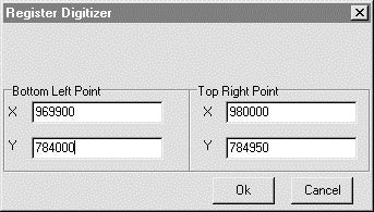
Figure 1: Registering your chart.
すると、プログラムより、ディジタイザを置き、チャートの左下、及び、右上のコーナー上でクリックするように促されます。 (数字2参照)一度、それらのポイントを登録すると、Symbolsツールバー、及び、プルダウンメニューがアクティブになります。
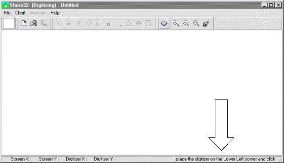
Figure 2: Follow registering instructions at the bottom ofthe program.
以上でチャートのデジタイジングが可能になります。実際にデジタイジングを開始するには、チャート上のディジタル化したい記号をク リックします。図3において、あなたは、海岸線をディジタル化するために「ライン」記号が記号ツールバーの中から選択されていることに気づくでしょう。別 の海岸線を作成するには、再び「ライン」記号を選択し直さなければなりません。そうしなければ、2つの岸線はつながれた状態になってしまいます。あるポイ ントを削除するにはポイント上で右クリックして"Delete"を選択します。
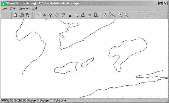
Figure 3: Digitizing shorelines with the "Lines" symbol.
チャートが完全でなるまで、記号を選択して、ディジタル化します。いったん、チャートをディジタル化したならば、File Saveをクリックし、名前をつけて保存してください。保存したファイルはDGWの拡張子がつきます。作成したファイルはDesign、または、Survey (図4参照)Hyplotで読み込むことが可能になります。
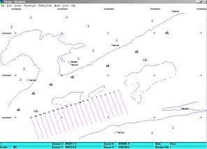
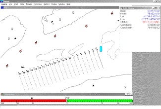
Figure 4: DGW file loaded in Design and Survey programs.
Qシングルビームの音速度補正について
補正はウォーターカラムでの離散的な間隔の音速度の測定された音速度プロファイルから始まります。
左下で示されるプロフィールは、感潮河川で1mおきに測定された典型的なサンプルです。
上層から下層までで約2.5%の変化があります。
右下に示される2つ目のプロファイルでは手計算により後に示す簡易計算により3点のみの音速度で作成されています。
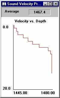
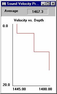
以下に示す表はおおよそのプロファイルを示します。
|
Layer End Depth (m) |
Layer Height – h (m) |
Sound Velocity – V (m / s) |
|---|---|---|
|
3 |
3 |
1449 |
|
9 |
6 |
1465 |
|
15 (bottom of cast) |
Unlimited |
1479 |
最後の層の高さは無制限となります。
計算例
測深器で音速度を1480 m/sに設定し、17.13 mが計測されました。 1mの喫水も測深器に入力します。上記の簡略化されたプロファイルを音速度補正として使用します。
最初に、深さは表面から底まで一方向の経過時間(1m当たり進むためにかかる時間)tに変換されます。:
t = 測深器の深度/ 測深器の音速度
t = 0.011575 seconds
プロファイルを使用した音速度補正にHypackでは各層におけるトラベルタイムを使用します。
最初の層では音波は3m進むのに0.002070秒かかります。(t= 層の厚み/ 最初の層の音速度 = 3/1449). その時間をトータルの所要時間から減じると0.009505秒残ります。
次の層では6m進のに音速度1465 m/sで0.004096秒かかります。2番目の層から海底まで要する残りの時間はトータルの時間より1番目と2番目の層にかかる時間を引いた結果となり 0.005409秒になります。残りの時間で音波が最後の層を進む距離はt*SV = 0.005409*1479 = 8.00 m
従って最終的な測深値は: 3 m (1番目の層) + 6 m (2番目の層) + 8 m (最後の層) = 17 m
従って音速度補正値は17.00 (真の測深値) – 17.13 (測深器の計測した測深値) = -0.13 m