HYPACKに関する質問
13.ボリューム---体積計算(Volumes)に関するFAQ
Qフィラデルフィア法体積計算(Philadelphia Volume Tests)[英語]
FAQ ID:Q13-1M
Tests were conducted on 1-2 March 2000 to determine the accuracy of the different volume techniques in HYPACK® Version 7.1, HYPACK® MAX (Cross Sections & Volumes) and HYPACK® MAX (TIN MODEL). Tests were run with multibeam data collected on a recent USACE Philadelphia project and with a test data set that allowed evaluation of all four box cut methods (Contour vs. Non-Contour; All vs. Shoals-Only).
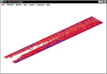
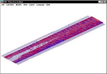
A sample channel with survey data was created and is shown below.
At the left toe-line the depth was above the project design depth. This meant the overdredge material on this side should be included in the Shoals-Only method. At the right toe-line, the depth was below the project depth. This meant that the overdredge material in this area would not be included in the Shoals-Only method.
On the left side, the depth passed through the design depth in the left box area. This means the contour dredge quantity for the left box area should be less than the non-contour dredge quantity. On the right side, the depth passes through the design depth in the "right of center" area. This means the contour dredge quantity for the right of center area should be less than the non-contour dredge quantity.
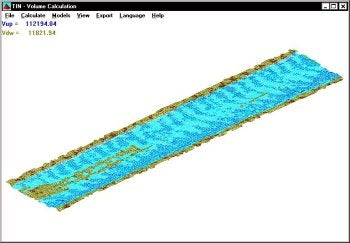
The points were first loaded into the HYPACK® MAX TIN MODEL program, along with the planned line file. The planned line file contained 11 lines at 100' spacing. Volume numbers presented below are in cubic feet.
TIN MODEL Tests
(Calculated quantities in black; Mathematical prediction in red.)
| Method | Dredge Left Box | Dredge Left Channel | Dredge Right Channel | Dredge Right Box | Overdredge Left Box | Overdredge Left Channel | Overdredge Right Channel | Overdredge Right Box |
|---|---|---|---|---|---|---|---|---|
| Non-Contour All |
3,125 |
900,000 (100%) 900,000 |
802,736 (99.99%) 802,736 |
0.0 (100%) 0.0 |
21,875 (100%) 21,875 |
200,000 (100%) 200,000 |
197,224 (100%) 197,222 |
2,776 (88.78%) 2,750 |
| Contour All | 3,125 (100%) 3,125 |
900,000 (100%) 900,000 |
802,736 (100%) 802,736 |
0.0 (100%) 0.0 |
12,500 (100%) 12,500 |
200,000 (100%) 200,000 |
188,800 (99.95%) 188,888 |
0.0 (100%) 0.0 |
| Contour Shoal-Only | 3,125 (100%) 3,125 |
900,000 (100%) 900,000 |
802,736 (100%) 802,736 |
0.0 (100%) 0.0 |
12,500 (100%) 12,500 |
200,000 (100%) 200,000 |
188,800 (99.95%) 188,888 |
0.0 (100%) 0.0 |
| Non-Contour Shoal-Only | 3,125 (100%) 3,125 |
900,000 (100%) 900,000 |
802,736 (100%) 802,736 |
0.0 (100%) 0.0 |
25,000 (100%) 21,875 |
1,100,000 (100%) 200,000 |
999,960 (529%) 197,222 |
0.0 (100%) 0.0 |
1. All of the Dredge quantities are mathematically correct.
2. The Contour vs. Non-Contour and All vs. Shoals-Only only effect the Overdredge Quantities
3. All of the Overdredge methods appear to be correct, with the exception of the Non-Contour - Shoals Only method. This method is reporting erroneous quantities and needs to be fixed.
HYPACK® 7.1 Tests
(Calculated quantities in black; Mathematical prediction in red.)
| Method | Dredge Left Box | Dredge Left Channel | Dredge Right Channel | Dredge Right Box | Overdredge Left Box | Overdredge Left Channel | Overdredge Right Channel | Overdredge Right Box |
|---|---|---|---|---|---|---|---|---|
| Non-Contour All |
3,109 |
900,000 (100%) 900,000 |
802,800 (100%) 802,736 |
0.0 (100%) 0.0 |
21,900 (100.11%) 21,875 |
200,000 (100%) 200,000 |
197,200 (99.99%) 197,222 |
2,800 (101.82%) 2,750 |
| Contour All | 3,109 (99.49%) 3,125 |
900,000 (100%) 900,000 |
802,800 (100%) 802,736 |
0.0 (100%) 0.0 |
12,000 (96.00%) 12,500 |
200,000 (100%) 200,000 |
189,000 (100%) 188,888 |
0.0 (100%) 0.0 |
| Contour Shoal-Only | 3,109 (99.49%) 3,125 |
900,000 (100%) 900,000 |
802,800 (100%) 802,736 |
0.0 (100%) 0.0 |
12,000 (96.00%) 12,500 |
200,000 (100%) 200,000 |
189,000 (100%) 188,888 |
0.0 (100%) 0.0 |
| Non-Contour Shoal-Only | 3,109 (99.49%) 3,125 |
900,000 (100%) 900,000 |
802,800 (100%) 802,736 |
0.0 (100%) 0.0 |
21,900 (100.11%) 21,875 |
200,000 (100%) 200,000 |
197,200 (99.99%) 197,222 |
0.0 (100%) 0.0 |
1. All of the quantity calculations were very close. The largest difference was 500 ft³ on the Left Box Overdredge for the Contour methods.
2. Wow! Pretty good.
HYPACK® MAX Tests
(Calculated quantities in black; Mathematical prediction in red.)
| Method | Dredge Left Box | Dredge Left Channel | Dredge Right Channel | Dredge Right Box | Overdredge Left Box | Overdredge Left Channel | Overdredge Right Channel | Overdredge Right Box |
|---|---|---|---|---|---|---|---|---|
| Non-Contour All |
3,145 |
900,000 (100%) 900,000 |
802,730 (100%) 802,736 |
0.0 (100%) 0.0 |
21,882 (100.03%) 21,875 |
200,000 (100%) 200,000 |
197,200 (100%) 197,222 |
2,780 (101.09%) 2,750 |
| Contour All | 3,145 (100.64%) 3,125 |
900,000 (100%) 900,000 |
802,730 (100%) 802,736 |
0.0 (100%) 0.0 |
12,545 (100.36%) 12,500 |
200,000 (100%) 200,000 |
188,800 (100%) 188,888 |
0.0 (100%) 0.0 |
| Contour Shoal-Only | 3,145 (100.64%) 3,125 |
900,000 (100%) 900,000 |
802,730 (100%) 802,736 |
0.0 (100%) 0.0 |
12,545 (100.36%) 12,500 |
200,000 (100%) 200,000 |
188,800 (100%) 188,888 |
0.0 (100%) 0.0 |
| Non-Contour Shoal-Only | 3,154 (100.64%) 3,125 |
900,000 (100%) 900,000 |
802,730 (100%) 802,736 |
0.0 (100%) 0.0 |
21,882 (100.03%) 21,875 |
200,000 (100%) 200,000 |
197,220 (99.99%) 197,222 |
0.0 (100%) 0.0 |
Wow! Even a little better than 7.1. These guys really know what they are doing!
ACTUAL DATA TEST: POOLE'S ISLAND RANGE C&D APPROACH CHANNEL
Volumes were calculated using the Contour - All method for single beam data using the HYPACK® MAX and HYPACK® 7.1 VOLUME programs. Data collected with the multibeam system was also processed and volumes computed with the TIN MODEL program. The results are shown below.
|
Method |
Material to Project Depth | Allowable Overdepth | Total Pay Place |
|---|---|---|---|
| Single Beam 7.1 | 81,742 cu.yds. (98.2% of MB) |
51,579 cu.yds. (101.0% of MB) |
133,322 cu. yds. (99.3% of MB) |
| Single Beam MAX | 81,747 cu. yds. (98.2% of MB) |
51,586 cu. yds. (101.0% of MB) |
133,333 cu. yds. (99.3% of MB) |
| Multibeam TIN MODEL | 83,219 cu. yds. | 51,084 cu. yds. | 134,303 cu. yds. |
1. The Single Beam techniques calculated slightly less "Material to Project Depth" and slightly more "Allowable Overdepth". The total material was less than 1% difference from the multibeam survey. This number is small for other tests done in the past. Typically, we have found the difference between single beam and multibeam surveys to yield normally up to 3% more material and sometimes as much as 6%. The above results are probably as close as you are going to see.
TEST: Matrix Cell Size vs. Dredge Quantities
The same edited multibeam data set was gridded at 1'x1', 5'x5' and 10'x10' cell sizes. The resulting XYZ data files were then run through the HYPACK® MAX - TIN MODEL program and volumes were calculated using the Philadelphia Box Cut method. The 1x1 data set contained 979,000 data points.
Computed volumes were:
|
Matrix Cell Size |
Normal Material (cu. yds.) |
Overdrege Material (cu. yds.) |
Total Material (cu. yds.) |
TIN & VOLUME Time to Finish |
|---|---|---|---|---|
| 1 x 1 | 83,173 | 50,969 | 134,142 | 7 hrs 15 min |
| 5 x 5 | 83,219 | 51,084 | 134,303 | 0 hrs 26 min |
| 10 x 10 | 83,305 | 50,978 | 134,283 | 0 hrs 3 min |
1. As shown by previous studies, the increased density of data points does not improve the results of the volume quantities. The longer processing time for dense data sets does not result in significantly different volumes.
QTINモデルにおけるフィラデルフィア法体積計算(Implementing of Philadelphia Post-dredge Method in TIN Model)[英語]
FAQ ID:Q13-2
Overview: Over the last couple of years, the use of multibeam echosounders for dredge payment surveys has become more common. Users have requested the ability of using all of the multibeam sounding data when computing volumes over an area.
Late last year, Lazar Pevac adapted the TIN MODEL program of HYPACK® MAX to be able to compute the volumes of a survey surface versus the template information in a planned line file (*.LNW). The Philadelphia District of the U.S. Army Corps of Engineers funded this work. The advantage of this method over previous methods was that it provided volume quantities for both dredge and overdredge templates and provided quantities for each pair of lines, breaking it down into left slope (or box), left of channel, right of channel, right slope (or box).
The last step of this development project was to be able to perform a pre-dredge versus post-dredge calculation in the TIN MODEL. Lazar has just completed this task and it is now available for interested users. It was not done in time for the 00.5 release CD, but is available from customer support. A description of the method is shown below.
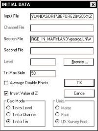
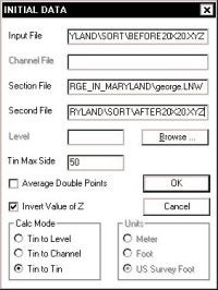
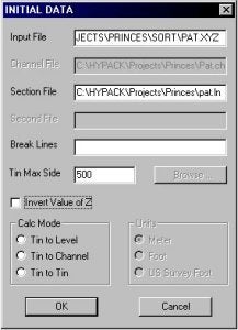
Start-up: There is nothing really new on starting the TIN MODEL program. When you are asked to enter your file information, you can specify a single file for a pre-dredge computation or two files for a pre-dredge versus post-dredge computation.
The figure (shown upper right) shows the layout for a single data file to be used in a pre-dredge computation. The figure (shown lower right) shows the layout for two data files and will result in a pre-dredge versus postdredge computation.
In both cases, we have included a planned line file (*.LNW: created in CHANNEL DESIGN). This planned line file will be used to determine the location of the lines and the dredge templates for each line.
In both cases we have checked the "Invert Value of Z" box. You want to do this if you are entering XYZ data. If I were using single beam data, I would not check this box. TIN MODEL will then correctly interpret the data.
You need to have the Tin to Tin method checked in the lower left hand corner in order to enter the Second File (Post-Dredge survey data).
If you are doing a Pre-dredge versus Post-Dredge computation, you should enter the filename with your Pre-Dredge data as your "Input File" and the filename with your Post-Dredge data as your "Second File".
Once you click the OK button, the TIN MODEL program will start with the first file and create the surface model. It will immediately go to the second file and create a surface model. Control will then be returned to the operator.
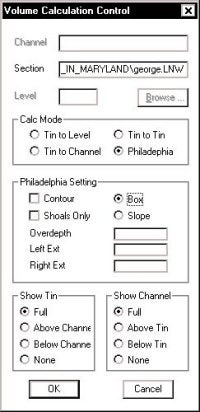
Set Method: The user should next go to the Calculate - Set Method menu item. There have been a couple of minor changes to the window.
The Planned Line file (*.LNW) specified during the initial window will appear as the "Section" file. This can be changed at any time before computing the volumes.
Under the "Calc Mode" frame, there is now just a Philadelphia choice. If you have specified only a single input data file, the program will provide a pre-dredge computation. If you have specified two input data files, the program will provide a pre-dredge versus post-dredge report. There is no way to over-ride this.
The type of Philadelphia computation can be either a Box or Slope. This check box has been moved into the "Philadelphia Setting" frame. If the user selects "Box", they must then enter the depth of the overdredge template beneath the design template, along with the extension distances for the box on the left and right sides.
If the user selects "Slope", all they have to specify is the depth of the overdredge template beneath the design template.
Once you have entered your settings, click OK to return to the main menu. Then click Calculate - Volumes to start the computation.
Computation Sequence: The TIN MODEL program is going to go through three computation stages:
- Compute Philly Volumes for Input File and Second Files .
- Generate a 3rd Surface that is the Differences Between Surfaces.
- Compute a Tin to Tin volume on the New Surface.
The image to the left shows the program after the first stage. It has computed the Philly volume information for each data set. The image on the right shows the program at the end of phase 2. It has computed a new surface by determining the separation between the original two surfaces.
In the figure to the right, the program has completed phase 3. This is the TIN-to-TIN computation. It is used to determine the total amount of material removed (regardless of the template) and the total of material "infilled" during the dredging process. These are areas where the bottom in the Post-Dredge data is shoaler than the Pre-Dredge data.
Before performing the TIN-to-TIN computation, the program "clips" the data to the borders of the Planned Line File (*.LNW). This is to prevent it from including material outside the area of interest in this computation.
The Pre-Dredge versus Post-Dredge report is then generated and can be viewed or printed from the Export menu. The report lists the quantities for each pair of survey lines. It shows the amount of material available after the pre-dredge survey, the amount of material remaining after the post-dredge survey and takes the difference between the two to obtain the material removed.
The summary for the computation is shown in the figure right. A description of each item is provided below.
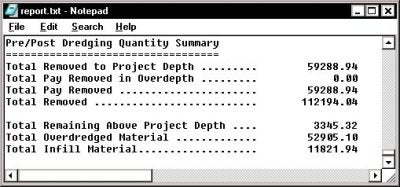
Total Removed to Project Depth: This is the total material above the dredge template from the pre-dredge survey minus the total material above the dredge template from the post-dredge survey.
Total Pay Removed in the Overdepth: This is the total material available in the overdredge template area from the pre-dredge survey minus the total material available in the overdredge template from the post-dredge survey.
Total Pay Removed: This is the sum of the above two items.
Total Removed: This is the total material removed between the pre-dredge and post-dredge surveys, without respect to the templates. It would include any material removed beneath the overdredge template that would not be included in the Total Pay Removed quantity.
Total Remaining Above Project Depth: This is the amount of material computed from the Post-Dredge survey that is above the design template. The pre-dredge survey is not used when computing this number.
Total Overdredged Material: This is the Total Removed less the Total Pay Removed.
Total Infill Material: This is the volume of material where the depth of the Post-dredge survey is shoaler than the Pre-dredge survey.
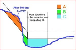
Qフィラデルフィア法による体積計算(HYPACK Volumes - Philadelphia Method)
FAQ ID:Q13-3
HYPACKで土量計算を行うフィラデルフィア法は、フィラデルフィアのアメリカ原子力委員会で特殊な状況の土量計算を扱うために開発されたものです。この方法では単一の測量での体積計算(Philadelphia Pre-Dredge)についてや、2回の測量による差分を計算(Philadelphia Post-Dredge)することができます。他の方法とこの方法との主な違いは、浚渫量をどのように扱うかというところにあります。
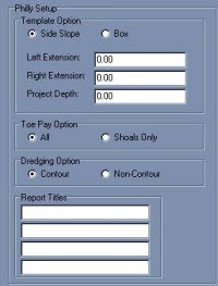
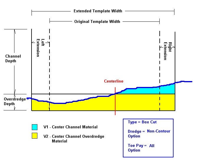
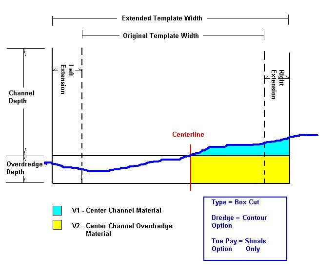
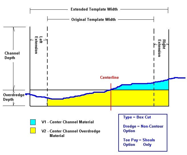
フィラデルフィア法は従来のSideSlope TemplateでもBox Templateでもどちらでも使えます。右下の図で示したように、Box TemplateではTemplate Option Flame(上図)内の「Left Extension」と「Right Extension」の入力することで法面まで距離を伸ばすことができます。同じフレームに新たな値を入力することで従来のchannel templateから水路の深度を変更することもできます。これらのオプションはBox Templateでのみ現れます。
Box Templateにおいて、プログラムではV1(水路の上の量)とV2(余掘り土量)を計算します。これらの量を「Left Extension」「Right Extension」「Left of Center」と「Right of Center」に分類します。
Toe Pay Optionでは拡張領域で浚渫量をどのように扱うかを決められます。「All」を選択した場合、拡張領域での全ての浚渫量が含まれます。「Shoals Only」を選択した場合、拡張領域で法線(上図の破線)における深度が水路の深度より浅い場合にのみ扱われます。
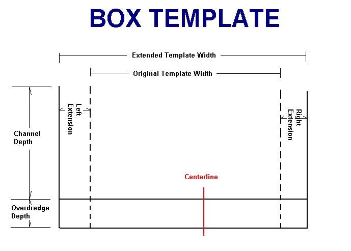
「Dredging Option」では「contour」「non-contour」を決められます。これは余掘り計算に含まれる土量に関係します。 「non-contour」を選択した場合、全余掘り土量が含まれます。「contour」を選択した場合、水路の深度より浅い部分の余掘り土量のみが含 まれます。
以下の4つの図は「Dredging Option」と「Toe Pay Option」をそれぞれの場合で4通りに組み合わせた場合を表しています。左拡張部と右拡張部の土量は水路中央部の土量と分けて表示されています。
Non-Contour & All (Box Cut)
Contour and Shoals Only (Box Cut)
Non-Contour & Shoals Only (Box Cut)
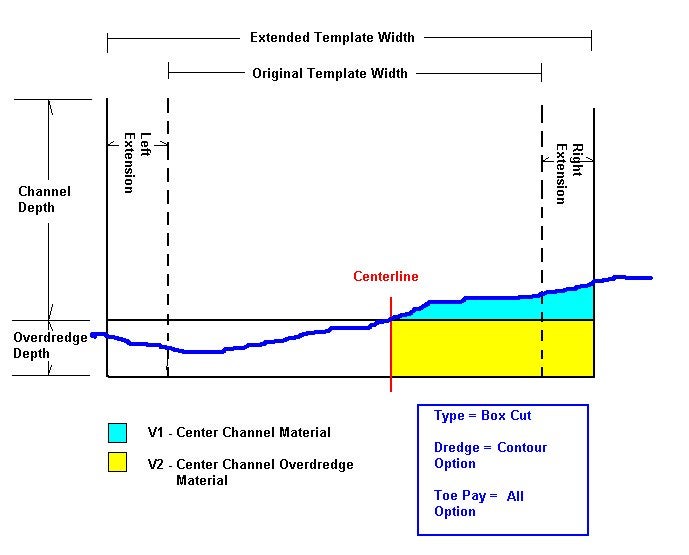
Contour & All (Box Cut)
フィラデルフィアメソッドセットアップ画面のSide Slope Optionでは、standard side slopeを使い、ボックスカット法で使われた左右拡張域・計画深度を削除します。Toe Pay Optionも必要ありません。唯一使用するオプションはDredging Optionの「contour」「non-contour」のみです。「contour」オプションでは計画深度より水路の深度が浅い部分の余掘り土量 のみ計算します。
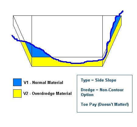
Non-Contour (Side Slope)

Contour (Side Slope)
(click an image to see the full size version)
QHypackTINプログラムの体積計算結果の検証(Buffalo Test)
FAQ ID:Q13-4
同一のXYZファイルに関して、HYPACK(TM)のTINモデルとInroads (Microstation) プログラムとで、ユーザー定義の表面の比較を行いました。結果は以下の通りになりました。
| Volumes (yd/cubed) | Area | TIN MODEL | Inroads | % Difference |
|---|---|---|---|---|
| LeftBank | Fill | 169,980 | 170,393 | 0.24 |
| Cut | 4,112 | 4,037 | -1.86 | |
| Center Channel | Fill | 319,945 | 320,007 | 0.02 |
| Cut | 57,578 | 57,593 | 0.03 | |
| Right Bank | Fill | 187,927 | 188,054 | 0.07 |
| Cut | 2,208 | 2,210 | 0.09 | |
| Total Channel | Fill | 677,852 | 678,454 | 0.08 |
| Cut | 63,898 | 63,840 | -0.09 |
Q体積計算におけるデータの質と量の関係(Quantity Versus Quality in Volume Computations)
FAQ ID:Q13-6
以下に示すのデータはHYPACK® MAXのTinモデルプログラムでPhiladelphia Post-Dredge法によって計算を行った場合の体積計算結果です。2種類の異なるサイズのグリッドデータを使用して計算をして比較しています。以下 に示すようにデータの数に比例して計算精度が上がるわけではないことがわかります。
つまり、データの数を適度に減らすことで余計な処理時間を削減できることになります。
| Material Type \Survey | Original Multibeam Data Set | 20' x 20' Binned Data Set | % |
|---|---|---|---|
| Dredge Left Box | 13,411 | 13,373 | 100.28 |
| Dredge Left Channel | 46,312 | 46,492 | 99.61 |
| Dredge Right Channel | 16,322 | 16,227 | 100.59 |
| Dredge Right Box | 7,250 | 7,135 | 101.61 |
| Overdredge Left Box | 2,956 | 2,963 | 99.76 |
| Overdredge Left Channel | 25,467 | 25,520 | 99.79 |
| Overdredge Right Channel | 24,935 | 24,974 | 99.84 |
| Overdredge Right Box | 2,957 | 2,962 | 99.83 |
| Total Dredge | 83,295 | 83,227 | 100.08 |
| Total Overdredge | 56,315 | 56,419 | 99.82 |
| Total Material | 139,610 | 139,646 | 99.97 |
QTINモデルプログラムの体積計算(Volumes Calculations in the TIN Model Program)
FAQ ID:Q13-7
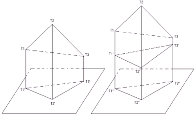
三角柱に関しての2つの簡単な数学の公式が、TINプログラムの土量計算の基本となっています。
式1:三角柱の端の線分が底面の三角形に垂直な時、その三角柱の体積は、下式(式1)で計算されます。
V = area( T1', T2', T3' ) * ( T1T1' + T2T2' + T3T3' ) / 3
Formula 1
三角柱の端の線分が底面の三角形に垂直でない時、その三角柱の体積は、下式(式2)で計算されます。
V = area(T1", T2", T3") * (T1T1' + T2T2' + T3T3') / 3
Formula 2
Tin対レベル計算法(Tin versus level volume calculation)
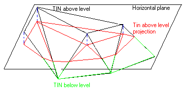
全ての三角形は、水平面の上部(above)と下部(below)に分けられます。体積は、公式を使い、平面の上部と下部に分けられて計算されます。(1)
Tin対チャンネル計算法(Tin versus channel volume calculation)
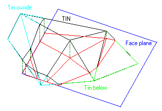
全ての三角形は、face planeの範囲で切断されます。face planeの内側の部分は、face planeの上部(above)と下部(below)に分けられます。体積は、公式を使い、face planeの上部と下部に分けられて計算されます。(2)
Tin対Tin計算法(TIN versus TIN volume calculation)
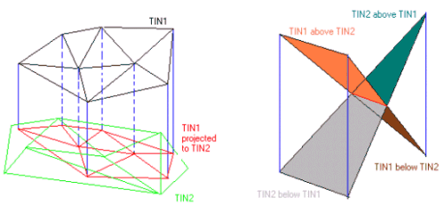
全てのTIN1の三角形は、TIN2に投影されます。新しく作られた TIN1'(TIN1がTIN2に投影されて出来た)のXY座標は、TIN1のXY座標と一致しています。Z値は、TIN2を使い補間されます。 TIN1(TIN1')の全ての三角形は、TIN1'よりTIN1が上(above)の部分とTIN1'よりTIN1が下(below)の部分に分けられ ます(TIN1' above TIN1とTIN1' below TIN1)。TIN1'より上のTIN1部分からなる各々の三角形は、関連するTIN1より下のTIN1'からなる部分とペアにされ、この体積は、(式 2)より計算されます。同じ手法がTIN1より上のTIN1'にも適用されます。
QTINモデルプログラムで特定の領域の体積計算を行う
FAQ ID:Q13-8
Advanced channel designプログラムにより作成されたchannelファイルを使用して特定の領域の土量計算をする事ができます。
<手順>
- [Utilities-Advanced Channel Design]を選択し、Advanced Channel Designプログラムを起動します。
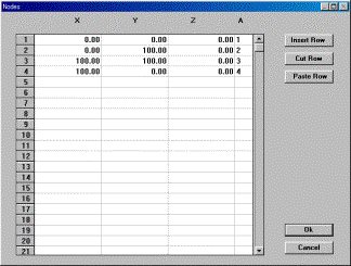
- [Edit-Nodes]を選択します。下図のようなウインドウが表示されますので、土量計算をする範囲を設定するためにXYZデータを入力します。(Zは、土量を比較したい面の高さを入力します。)Aに上から1,2,…と下図のように入力し、[OK]をクリックします。
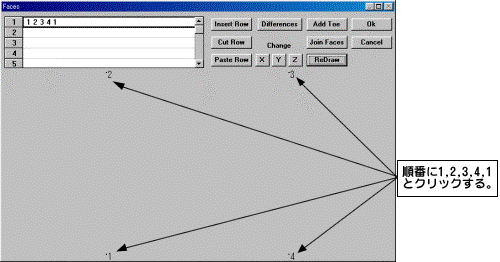
- [Edit-Faces]を選択し、Face editorを起動します。[ReDraw]をクリックすると、下図のように画面の下部に番号が表示されるので、順番に番号の上をクリックします。左上の 欄に順番に1,2,3,4,1(スペース区切り)で自動的に入力されます。このとき最初と最後の番号を同じ番号にします。[OK] をクリックします。
(注意)
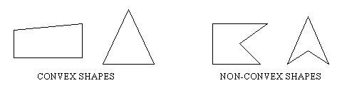
フェースが3ポイント以上で構成されている時、体積計算プログラムが正常に機能するには、フェースが凸型でなければなりません。非凸型形は、2つ以上の凸 形で構成されていますので分割して計算してください。
- [View-2D View]を選択し、形を確認します。次に[File-Save]をクリックしてchannelファイル(*.chn)を保存します。
- [Final Product-Tin Model]を選択し、Tinプログラムを起動します。
- Input Fileを選択し下図のように、作成したChannel Fileを選択し[OK]をクリックします。
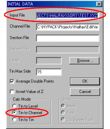
- [Calculate-Set Method]を選択し、下図のように[Cal Mode]をTin to Channelに設定します。[OK]をクリックしメイン画面に戻ります。
- [Calculate-Volume]を選択し、土量を計算します。
QTINモデルでチャンネル(CHN)ファイルを利用して体積計算する
FAQ ID:Q13-9
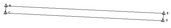
この例で計算に使用されるチャネルは、上の図において示されるものです。A-B-D-C-A多角形の中に含まれるエリアは、深度8.0mにあり、A-B toeラインから0.0mに達する10:1のサイドスロープがあります。同様に、C-D toeラインから0.0mに達する10:1のサイドスロープがあります。
Tin ModelにCHNファイルを使用する
この方法ではTIN MODELプログラムにおいてボリュームを計算するために、ADVANCED CHANNEL DESIGN ( ACD )プログラムにおいて作成されたチャンネル(*.CHN)ファイルを使用します。ACDプログラムによってユーザーは‘ノード’ポジション(上のA-B-C-D )を入力し、その後、どのようにノードを‘フェース’に結合するかを指定することが可能となります。ACDプログラムユーティリティは、‘Top of Bank’ライン、toeライン上のノードとサイドスロープを生成することができます。
ACDプログラムを開き、File-Newを選択
Window-Nodesを選択し、X-Y-Zの対等の情報を入力しなさい。
以下の図は、スプレッドシート及び、プランビューにおけるノードを示します。
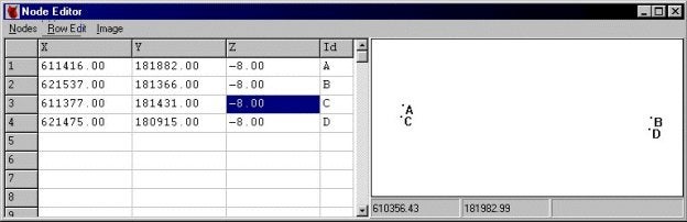
Tin ModelプログラムではZ軸の上方を正として計算を行うため、上記の例では深さを–8.00と入力しています。
Nodes – Saveを選択し、このウィンドウを閉じます。
Window – Facesを選択すると、どのようにノードをつなぐかを指定し、サイドスロープフェースを自動的に生み出すことが可能となります。
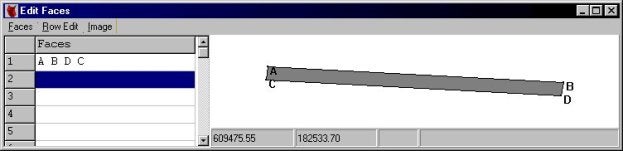
入力が終了すると自動的にこの面を閉じるため、スタートと同じノード、最後に指定する必要はありません。
5.北サイド(A-B)に沿って‘ side slope ’
エリアを作成します。
Faces – Add Toes を選択します。ポリ‐ラインA Bを使用し、10:1で深度0.00 (表面のレベル)まで傾斜していることを入力します。
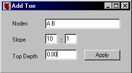
プログラムは、bankラインのトップを計算し、自動的にノードA、Bに結合した新しいフェースを生成します。bankラインのトップは、常に指定されたポリ‐ラインの左側に生成されます。下の図は、ノード‘5_’ (西エンド)、及び、‘6_’ (東エンド)、及び、フェースA B 6_ 5_’を生成された例です。
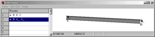
6.南サイドに沿ってサイドスロープエリアのための同じ手続きを繰り返します。
Faces – Add Toesを選択後、新しいノードは常に左側に生成されるのでNodes欄には“D C”の順で入力します。
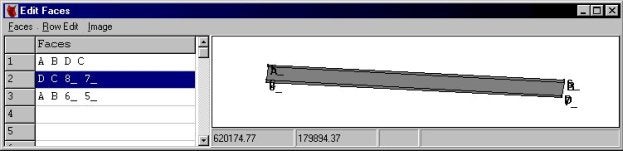
7.7. Faces – Saveを選択、Faces – Exitを選択します。
以下に示す図はHYPACK上での作成したチャンネルファイルとその西端の拡大図です。:
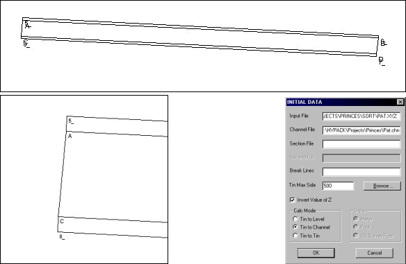
8.8.TIN MODELを起動し、TIN対Channelボリューム計算をする設定を行います。
これによって作成済みのCHNファイルの名前を入力することが可能となります。同じく計算対象となるXYZデータファイルの名前を入力し、Invert Z ValuesをチェックしZ値を反転させます。
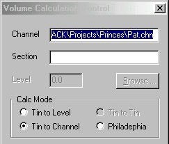
9.9.Tinが生成されたならば、Calculate – Set Methodを選択し、モデルとCHNファイルの体積を計算していることを確認します。
10.10.Calculate – Volumesを選択ます。
プログラムは、チャネルの上部、下部の体積を計算します。バージョン00.5Bの TIN MODELプログラムでは、各フェース毎に分離して計算を行います。これによって左のサイドスロープエリア、センタチャネルエリア、及び、右サイドスロープエリア上での体積を求めることが可能となります。
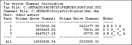
上図において示されたレポートにおいて、Volume Above Channelが埋め立てなければならない体積、 Volume Below Channelが浚渫しなければならない体積です。
この場合、我々は、センタチャネル( A B D C )に2,421,377.99 m³、右サイドの上で( D C 8_ 7_)70,651.68 m³、左のサイドの上で3 0,772.85 m³、浚渫する必要のある体積の総計は、2,522,802.51 m³となります。
Qクロスセクションでライン(LNW)ファイルを利用して体積計算する
FAQ ID:Q13-10

この例で計算に使用されるチャネルは、上の図において示されるものです。A-B-D-C-A多角形の中に含まれるエリアは、深度8.0mにあり、A-B toeラインから0.0mに達する10:1のサイドスロープがあります。同様に、C-D toeラインから0.0mに達する10:1のサイドスロープがあります。
Tin Modelプログラムで断面を切る
Tin Modelプログラムで断面を生成するにはあらかじめ測線(*.LNW)ファイルを作成しておく必要があります。
TIN MODELプログラムを起動します。初期設定の第ログでInvert Z ValuesをチェックしZ値を反転させます。Section File欄にあらかじめ作成した測線ファイルを入力します。その他の設定は通常Tin Modelを作成する場合と同様です。
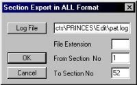
Export – All Formatを選択します。Log File欄に作成する断面のファイル名を入力します。このルーチンは、各測線に毎にHYPACKのAllFormatのデータファイルを作成し、それを現 在のプロジェクトの/Editディレクトリに保存します。
各ラインは、例えばcenterline (に沿ってそのラインに基づく名前で保存されます。(‘0+00’、‘2+00’、‘4+00’、…):
|
ライン名 |
ファイル名 |
|---|---|
|
0+00 |
0+00.ALL |
|
2+00 |
2+00.ALL |
|
4+00 |
4+00.ALL |
|
…… |
………… |
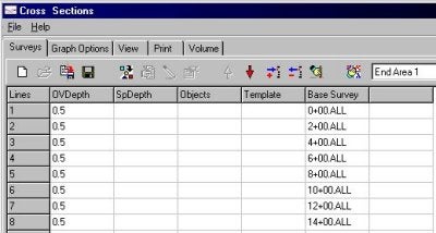
TIN MODELプログラムを終了し、CROSS SECTIONSプログラムを起動します。Surveyタブにおいて、Tinモデルで作成された断面のカタログファイルの名前を入力します。するとカタロ グが含むファイルが読み込まれ、図において示されたように、順番にそれらをリストされます。同じく0.5mの余掘り値を入力し、計算方法としてAEA1 Methodを使うように設定します。
その結果生じる断面は、下のスクリーンキャプチャにおける14+00の間で示されます。
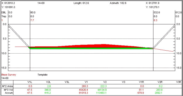
ボリューム量の要約は、下図で示されます。
以下に示される表は各計算方法による結果の比較です。
|
ケース1 :Tin ModelにCHNファイルを使用 |
2,522,802.5 m³ |
|---|---|
|
ケース2 :Tin ModelにLNWファイルを使用 |
2,517,678.5 m³ |
|
ケース3 : CROSS SECTIONSにTin Modelで生成された断面を使用 |
2,500,658.5 m³ |
この方法で計算を行うと他の2つの計算結果に比べ17,000 m³(約0.7%)少ない結果となっています。
おそらく、この差異は、いくつかのラインのエンドの水深データの希薄なデータが存在することによると思われます。
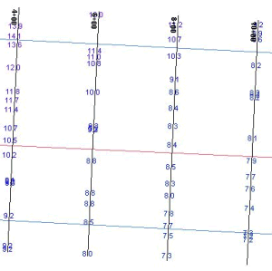
上図は、2、のラインのために作成された水深測量を示します。
TIN MODELは、TIN三角形の脚が測線(ライン)と交わる全てのロケーションで測深データを作成します。ラインがスロープのトップを越えて伸びていない場 合、ラインエンドでギャップから時折離れたものとなります。(ライン端の直下の基準面の深さを採用します。)これが原因で体積計算の際の誤差となることが あります。
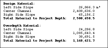
ラインを延長して再計算した結果は下記の通りです。:
|
左サイドスロープ: |
30,772.7 |
|---|---|
|
チャネルの中心: |
2,420,966.5 |
|
右サイドスロープ: |
68,232.5 |
|
計画水深に対する体積: |
2,519,971.7 |
結果は、非常に首尾一貫したものとなりました。:
|
ケース1 :Tin ModelにCHNファイルを使用 |
2,522,802.5 m³ |
|---|---|
|
ケース2 : Tin ModelにLNWファイルを使用 |
2,517,678.5 m³ |
|
ケース3 : CROSS SECTIONSにTin Modelで生成された断面を使用 |
2,519,971.7 m³ |
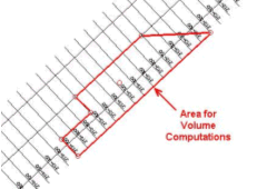
QEnd Area法体積計算の断面間の距離の決め方(Determining Distance Between Lines for Average End Area Volumes)
FAQ ID:Q13-11
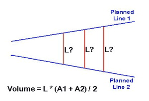
計画測線が平行である場合、測線間距離の決定はとても簡単です。計画測線が平行でない場合に問題が生じます。二本の測線間の距離決定は土量に影響を与えます。
例えば 、右図でArea1及びArea2(各々の計画測線上の面積)は、定数であり、計算結果の土量は、Lの値(測線間距離)が大きくなるにつれ増加します。
もし私が、港湾管理機関の人であれば、計算結果の土量を最少にするLの値を選び土量が少なくなるよう試みるでしょう。反対に、私が浚渫工事会社の人 であった場合、正しいLの値は出来るだけ大きな値に出来るものを主張するでしょう。双方の主張のバランスをとる為に、平行でない測線に対する、Lの値の決 定法が必要です。この章では我々が使用している所をみた、いくつかの方法について考察しHYPACK® MAX で使用されている方法について説明します。
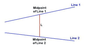
Midpoint Method(中点法)
: 一つの方法は、測線の中点を結び測線間距離を決めます。右図の赤線がこの方法により決められた距離を示しています。
一方の測線がもう一方の測線にたいしてオフセットされていない状態の時には、この方法は良い近似を示す傾向があります。
右図にこの方法を使用しないであろう状態の例を示します。短い測線(Line1)と長い測線(Line2)が あるとします。各測線の中点は、測線に対して直行していません。この方法で計算されたLの値は二本の平行な測線の距離100’よりずいぶんと長くなってし まいます。これが結果として土量を多く見積もってしまいます。
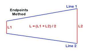
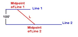
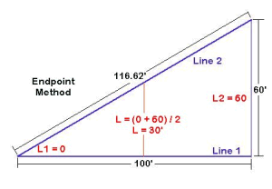
Endpoint Method(端点法)
: その他の方法は、各測線の端点を結んだ線分を平均する方法です。右図では、Lの値を得る為にL1とL2を平均します。
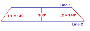
この方法は、測線が同じ長さの時はかなりうまく機能します。うまくいかない場合は、下図に示すように一方が他方より長い時です。
この図で平行測線間の距離は100’です。しかし、Line1はLine2よりずっと短いです。この例では、 各端点間の距離は140’です。この値を使用するとこの部分で40%多く土量を計算してしまいます。このような場合、この方法を使用する事は不正と思われ てしまうでしょう。
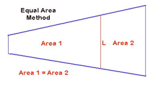
Equal Area(等面積法)
: 最近我々がみた方法は線の両側の各面積を等しくするようにLの値を選択する方法です。
図で示すように、Lの値は、左側の面積(Area1)と右側の面積(Area2)が等しくなるように選択されています。
この方法は、おそらくその面積を通る線によって等しくされた面積”centroid”を決める為に開発されたのであろう。例の部分にて、この方法が一般にこの部分の土量を多く見積もってしまう事を示しましょう。
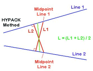
HYPACK® MAX Method(HYPACK® MAX法)
: 数年前多くのテストを経て我々は土量計算に使用する測線間距離決定の為のこの方法を提案しました。
Line1の中点を起点とし、Line2へ直行するように垂線をひきます。これをL1と呼びます。次にLine2の中点を起点とし同様に垂線を引きます。これをL2と呼びます。続いてLの値を決める為に、L1とL2の平均をとります。
この方法により、とても良い測線間距離の近似計算をほとんど全ての場合について行えます。
実例
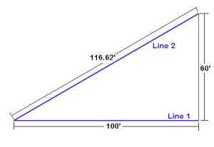
: これらの方法を試し計算された土量の差を示す為に以下の例を示します。
Line1とLine2は左の点が接しています。Line1は100’の長さでLine2は116.62’の長さです。右端で60’離れています。これは右の三角形を形作ります。
入力した計画面より1’海底が上にあるとみなします。Line1上の面積は、100 ft² でLine2上の面積は116.62 ft²になります。
数学的に三角形の面積は3,000 ft²です。海底面が計画面より1’上にあるので数学的な土量は3,000 ft³です。
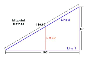
例: Midpoint Method(中点法)
: 各線分の中点を使用すると、L値は30’になります。これを平均断面法の公式にあてはめます。
V = L * (A1 + A2) / 2
V = 30. * (100. + 116.62) / 2.
V = 3,249.30 ft³ (+8.3%)
例: Endpoint Method(端点法)
: この方法を使用し、二本の計画測線、各々の端点間距離を計算します。左側の距離は0’であり右側の距離は60’です。従って平均の距離は30’です。この結果は中点法で使用した距離と同じになりました。
V = L * (A1 + A2) / 2
V = 30. * (100. + 116.62) / 2.
V = 3,249.30 ft³ (+8.3%)
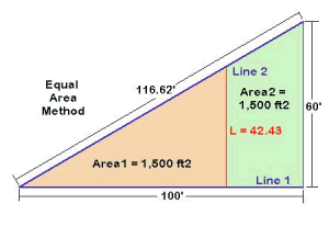
例: Equal Area Method(等面積法)
: この方法では、Area1の面積(三角形)とArea2の面積(台形)が等しくなるようにLの値を計算しなければなりません。ちょっとした代数と幾何学を使いL値が42.43'であり、両面積は1,500 ft².になることが判明します。
この結果を平均断面法の公式にあてはめると下記答えがえられます。V = L * (A1 + A2) / 2
V = 42.43 * (100. + 116.62) / 2.
V = 4,595.59 ft³ (+53.2%)
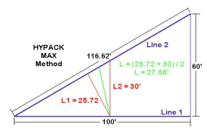
例:HYPACK® MAX Method(HYPACK® MAX法)
: Line1の中点よりLine2へ垂線をひくと、その長さL1は25.72'です。Line2の中点よりLine1へ垂線をひくと、その長さL2は30'です。L1とL2の平均をとると、27.86’になります。
平均断面法の公式にあてはめると下記の答えがえられます。
V = L * (A1 + A2) / 2
V = 27.86 * (100. + 116.62) / 2.
V = 3,017.5 ft³ (+0.5%)
要約すると、HYPACK® MAX法によって計算されたL値が、数学的事実に最も近い平均断面土量となりました。これは、他の方法より我々の方法が優れていることを示す、我々が行ってきた数々の例中の単なる一例にすぎません。
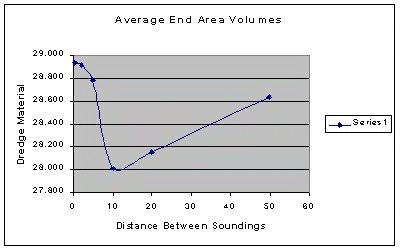
Qデータ密度がAverage End Area法体積計算に与える影響(Effect of Along-Line Spacing of Single Beam Data on Volumes Calculations)[英語]tion of Average End Area Volumes
FAQ ID:Q13-12M
Well, that's a hell of an impressive title. If I were to tell you of a way that you could make $20,000 without any additional effort would you be interested? If I tell you how, would you give me half? If your answer to the last two questions is "Yes", then read on. Otherwise, go look at the cartoon.
HYPACK® can collect every sounding that comes out of your echosounder. If your sounder is updating at 15 times per second and your boat is traveling at six knots, this means you will have a sounding every 8" along your planned line.
Now, when you go to compute volumes, should you use all of these soundings or should you "thin" the data by using one of the sounding selection programs?
In preparation for my Volume Seminar at the 2001 U.S. Hydrographic Conference (21-24 May 2001 - Sheraton Norfolk Waterside Hotel - details at www.thsoa.org) I took a single beam data set and did some tests to determine how the volumes compared when I thinned the data using different spacings.
Below is a plot, taken from a capture of the CROSS SECTIONS program. The original survey data is spaced about every 8" and is in black. I then ran the data through the MAPPER program, using a 20' x 20' matrix and saved the point "Closest to the Center" of each cell to an XYZ file. [It's a little more complex, as I then took the XYZ file result from MAPPER, ran it into the TIN MODEL and then cut sections through it to get it back into EDITED ALL format so I could then load the results back into CROSS SECTIONS.] The soundings at 20' spacing are shown in red on the picture below.

Visually, there isn't a whole lot of difference between the two sections. The file with the 8" spacing moves above and below the file with the 20' spacing, but it's not evident what the effect will be on the volumes.
I ran volume quantities for the entire channel, once for the 8" data and again for the 20' data. The 8" data had almost 3% more material. I then ran some more tests, sampling the data at 2', 5', 10', 20' and 50' spacing to see the result. The computed volumes are summarized in the table and graph below.
| Spacing | Dredge Material (cubic yards) |
% of original |
|---|---|---|
| 8" | 28,938 | 100 |
| 2' | 28,911 | 99.9 |
| 5' | 28,782 | 99.5 |
| 10' | 28,009 | 96.8 |
| 20' | 28,151 | 97.3 |
| 50' | 28,630 | 98.9 |

The test conducted on this data set was repeated on a different data set with almost identical results.
So, if I want to maximize my volume quantities, I will use every data point in the sounding set. If I want to minimize my volume quantities, I will thin the data every 10' along the line.
The difference in this data set between those two approaches is 929 cubic yards. At $22/yard, that comes to a savings of $20,438.
Qフィラデルフィア法体積計算結果について(Philadelphia Pre- and Post-Dredge Reports)[英語]
FAQ ID:Q13-1M
There have recently been a lot of questions as to the meaning of items in the Philadelphia Pre-Dredge and Post-Dredge Reports of the CROSS SECTIONS program. The purpose of this article is to examine those items and to provide an explanation of differences between the Pre-Dredge and Post-Dredge numbers. I ran the Philadelphia Pre-Dredge method using a Before-Dredge (befores) and an After-Dredge (afters) data sets. I then ran the Philadelphia Post-Dredge method using both data sets.
Philadelphia Pre-Dredge Report - Befores
Let's first take a look at a section of the Philadelphia Pre-Dredge Report. If you get down to the station-by-station numbers, you'll see something like the following for your data set:
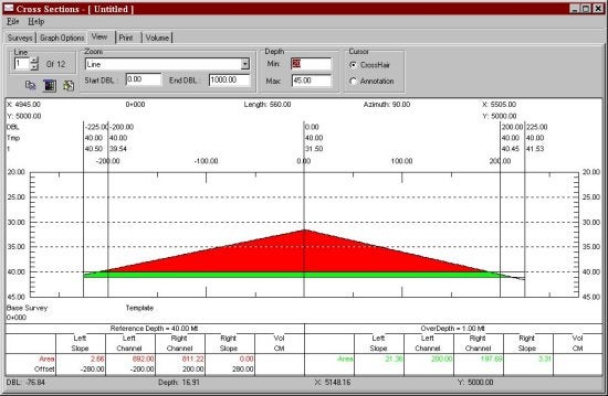
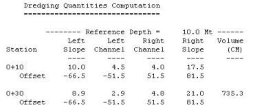
For the Station 0+10, the Left Slope has 20.0m² of material; the Left Center Channel has 13.8m² of material; the Right Center Channel has 8.6m² and the Right Slope has 15.3m².
The Offsets refer to the distance (from the centerline) to each feature. The Top of the Left Slope is -66.5m (left 66.5) from the centerline; the Left Toe Line (start of side slope) is -51.5m (left 51.5); etc.
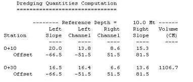
For the Section 0+30, the information is repeated. Since our lines in this test are 20m apart, we can create a simple table to determine the volumes for each section. Volume = (Area1 + Area2) * Dist / 2.
| Section/Area | Left Slope Area | Left Channel Area | Right Channel Area | Right Slope |
|---|---|---|---|---|
| 0+10 | 20.0m² | 13.8m² | 8.6m² | 15.3m² |
| 0+30 | 16.5m² | 16.4m² | 6.6m² | 13.6m² |
| Volume | 365m³ | 302m³ | 152m³ | 189m³ |
| Total Volume | 365 + 302 + 152 + 189 = 1108m³ | |||
The difference between the report's 1106.7 m³ and the 1108 m³ in our table is that the areas in the report are only reported to 0.1 precision but are maintained at a higher precision inside the program.
The same can be repeated for the numbers in the Overdepth area of the report. These numbers are located in the right-hand side of the report and contain the areas and volumes of material in the Overdepth area.
Philadelphia Pre-Dredge - Afters
I then ran the data files from the After-Dredge survey, using the same Philadelphia Pre-Dredge report. This will be handy later on when comparing numbers in the Philadelphia Post-Dredge Report.
In this case, if I repeat the computation done above, I get the volume between the two sections to be 736 m³. This is almost equal to the value in the report, the difference being that I am using the areas that have been rounded to the nearest 0.1m².
So far, so good.
Philadelphia Post-Dredge Report - Befores and Afters
Now let's take a look at the report from the Philadelphia Post-Dredge method.
There are two sets of "areas" reported for each section.
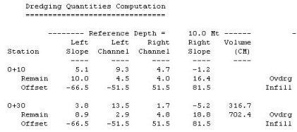
The top line (5.1 9.3 4.7 -1.2) represents the amount of material (m²) that has been removed in each segment. It determines this number by first determining where the two data sets overlap. It then computes the available area in Survey 1 (S1) and the available area in Survey 2 (S2) and computes the area of material removed (S2-S1). The negative number (Right Slope) in our example reflects that material has actually been added in the Right Slope area in the area of comparison.
The second line (10.0 4.5 4.0 16.4) represents the amount of material that is still available in the section. You will notice that these numbers are slightly different than those reported at the top of the page in the Philadelphia Pre-Dredge report using the After-Dredge data (10.0 4.5 4.0 17.5). The reason for that is that the Philadelphia Post-Dredge will only report area where there is overlapping data on both surveys. [This is also true for the material that has been removed.]
Let's take a close look at the pre-dredge and post-dredge sections for line 0+10.
If we take a close look at the right side slope (the area from 51.5 to 81.5 on the right of the graph), the line from your before-dredge survey is displayed in black and the line from your after-dredge survey is displayed in blue. The black line stops right at the 5.0m level. For the Philadelphia Post-Dredge method, all area computations will stop at this point for both surveys. (Even though there is information in the after-dredge survey that is not going to be used.)
The post-dredge line originally reported 17.5m² of area available on the Right Slope in the Philadelphia Pre-Dredge report. In the Philadelphia Post-Dredge report, there is only 16.4 m² of area available. This is because it has not included the 1.1 m² of material that occurs beyond the point where the before-dredge survey ended.
Looking again at the Philadelphia Post-Dredge Report:
The value of 316.7 m³ reflects the amount of material that was removed between station 0+10 and 0+30. Once again, this is only computed where both data sets overlap.
The value of 702.4 m³ is the amount of material that remains to be removed (once again where we compare only areas where the two data files overlap).
In the Philadelphia Pre-Dredge report (using the after-dredge data file), it reports 735.3 m³ of available material. We have lost 32.9 m³ because the before-dredge survey did not overlap all the way across with the after-dredge survey. Note: If the after-dredge survey did not extend all of the way across and the before-dredge did extend all of the way across, the reported volumes in the Philadelphia Post-Dredge report would also be smaller than in reality.
If I take the available material generated by running the before-dredge and after-dredge surveys (separately) through the Philadelphia Pre-Dredge report and take the difference, I get 371.4 m³ (1106.7 - 735.3), versus the 316.7 m³ reported above.
Which value is correct? They are both correct. It is just that the Philadelphia Post-Dredge method is designed to only compare areas where there is over-lapping survey data.
Note: The Average End Area 3 method handles things differently. It computes all of the area under the pre-dredge survey and then computes all of the area under the post-dredge survey and then takes the difference without worrying about where the two data sets overlap. This is the major difference in the reported quantities between the two methods.
Philadelphia Post-Dredge Report - Summary
Finally, lets take a look at the Philadelphia Post-Dredge Report.
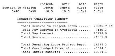
The top item is Total Removed To Project Depth. This is a sum of all of the material removed above the design template. It is computed by adding all of the reported quantities in the report. It would take the quantity between lines 0+10 to 0+30 (316.7 m³) and add it to the quantity between lines 0+30 to 0+50 (265.1 m³) and add it to the quantity between lines 0+50 to 0+70 (187.3 m³), etc.
The item Total Pay Removed In Overdepth is the sum of all of the material reported removed between the design template and the over-depth template. It's the same as above, repeated using the "over-depth" numbers in the right hand side of the report. (173.9 + 163.7 + 129.9 …..)
The Total Pay Removed is the mathematical sum of the above two item.
The Total Removed is the Total Pay Removed plus the material removed beneath the Overdepth template. In our test case, we have actually added material beneath the Overdepth template, so the Total Removed is less than the Total Pay Removed. There are no numbers in the report to confirm this. You can only examine the sections in the areas where the depths are less than the Overdepth template. It's very useful to plot out both sections on top of each other. Please look at the section below.
If you take a look in the area where the data is deeper than the over-depth template (center channel), the before-dredge survey (black) is deeper than the after-dredge survey. In effect, there is now more material in the center of the channel, although it is still beneath the over-depth template. This is what is causing our Total Removed to be less than our Total Pay Removed. This happens very rarely.
The Total Remaining Above Project Depth is just the sum of all of the remaining volume quantities for each pair of sections from the report below. In our case it would be 702.4 + 671.9 + 469.4 +…..
The Total Overdredged Material is the mathematical difference between the Total Removed minus the Total Pay Removed. Normally, it is used to show how much extra material the contractor removed beneath the over-depth template. Since we get a negative, it shows how much material has accumulated beneath the over-depth template in your project.
The Total Infill Material is the sum of all material where the pre-dredge survey was deeper than the post-dredge survey. There are no specific numbers provided in the report to verify this number.
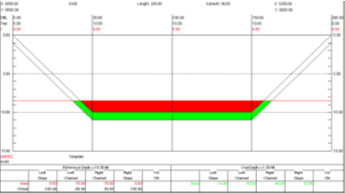
Qクロスセクション(断面と平均断面計算)プログラムにおけるテンプレートの使用(Custom Templates in Cross Sections and Volumes)
FAQ ID:Q13-14
最近、色々な形状の水路をメンテナンスする顧客が出てまいりました。(下図参照)
彼らは、HYPACK MAXで水路の型と計画測線を自動で作成してくれるCHANNEL DESIGNを利用します。CHANNEL DESIGNは水路の深度とサイドスロープの情報に沿って、左トーライン・センターライン・右トーラインの情報を入力するだけでLNWファイルが自動的に作成することができます。
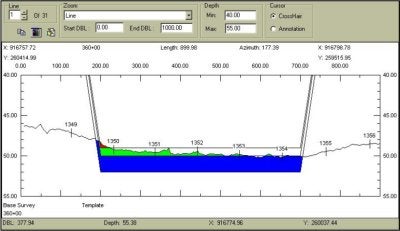
測量し編集されたデータをCROSS SECTIONSプログラム実行時に水路の体積計算を行うために読み込みます。断面図の例を下に示します。取り除くべき土の総量は320000yd3以上でこのプロジェクトでの量を超えています。
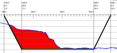
取り除くべき土の総量を減らすため、この機関では注目するエリアを縮小することにしました。彼らは取り除くべき部分のラインを左トーラインより30m内側に変更しました。つまり水路のセンターライン沿いに似たラインを作ることにしました。(下図参照)
この情報はプロットされ、元のラインから両岸の人工エリアまでの距離が測られました。
元のデータファイルをCROSS SECTIONプログラムでロードします。Template Editorを使い、新しい水路断面の形情報を入力しセーブします。この手順を各測線で繰り返します。
下図の例では、4 点のテンプレートがあります。最初の点は中心線の表面(深度0)から191.7mの位置にあります。2番目の点はそこからまっすぐ下29mで、新しい水路 の左端は井戸のように垂直になっています。3番目の点は中心線から341mで深さは29m、4番目の点はそこからまっすぐ上で、341mの位置です。
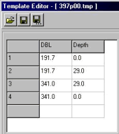
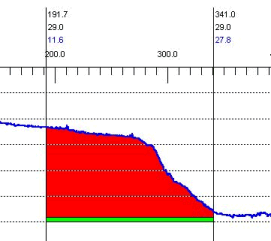
このテンプレートと水路断面は下図のように表されます。(CROSS SECSIONS – Viewerより) 両端が垂直の井戸のようになっているため、V1L、V2L、V1R、V2Rの量はありません。全体の土の量はV1とV2です。
この手順を全測線に対して繰り返します。単純な作業でこの例では30分くらいかかるでしょう。
もし水路が同じ断面をしているようならば、1つのテンプレートだけで水路全体をカバーできるでしょう。
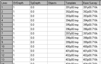
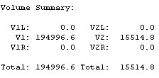
全部のテンプレートができあがったら、全土量を確認します。下図のように示されます。
QJacksonville法体積計算(Modification of Jacksonville Post-dredge Method to Compute Boxcuts)[英語]
FAQ ID:Q13-15M
Fran Woodward of the USACE Jacksonville District recently got in touch with us and requested some changes in the Jacksonville Post-dredge computation method that currently exists in the CROSS SECTIONS program. These changes include:
- The ability to compute the overdepth material using either ALL or Contour dredging methods.
- The ability to exclude the side slope areas from all computations.
- The ability to compute box cuts that provide for side slope material to slough off into voids created beneath the overdepth template around the toes.
There are now two options for the computation of overdepth material. These are "All" and "Contour". Using the "All" option, all material in the area between the design template and overdepth template will be computed. Using the "Contour" option, overdepth material will only be computed where the measured depth is less than the design template. This is identical to the technique used in the Philadelphia Methods of CROSS SECTIONS and the TIN MODEL.
The big change is the revised computation of box cut quantities. Take a look at the figure.
Digging precisely on the side slope is a hard job. In areas where the bottom material is soft, contractors are sometimes allowed to dig deep holes at the toe locations, with the idea that the material on the side slope will fall into the holes created.
In a soon-to-be released version of the CROSS SECTIONS program (it didn't make the 00.5B release), the following quantities will be computed separately for the left side and right side of each pair of survey lines.
A =The remaining side slope material from the after-dredge survey that is above the overdepth template. This will include all material above the design template and between the design and overdepth templates. This material is orange in the above figure.
B =The void present from the toe line outward from the centerline where the after-dredge survey is deeper than the overdepth template. This material is green in the above figure.
C =The void present from the toe line inward towards the centerline a user-specified distance where the after-dredge survey is deeper than the overdepth template.
These areas are computed for each line. [Separate areas are computed for the left and right sides of the channel. The program then uses the Average End Area formula to compute the volume of material contained in the A, B, and C areas between each pair of survey lines.
The Box Cut Volume is then determined by using the following rule:
If A > (B + C) then Box Cut Volume = B + C
If A < (B + C) then Box Cut Volume = A
For example, if I have 80 yd³ of available material remaining on the side slope and I have dug a void of 200 yd³, I'm only going to get credited 80 yd³. [I can't have more material fall into the hole than actually exists.]
Likewise, if I have 150 yd³ of available material on the side slope and I have dug a void of 75 yd³, I'm only going to get credited 75 yd³. I'm only going to get credit until the void is full.
Q新しい平均断面体積計算方法(Norfolk Volume Method Added to HYPACK® MAX)[英語]
FAQ ID:Q13-16
As a result of a contract with USACE-Norfolk, Coastal Oceanographics has added the ‘Norfolk’ Method as an option in the volume computation routines of the CROSS SECTIONS program. The Norfolk method is based on the average end area method of computing quantities.
It computes the entire volume above three user defined levels. In the example shown below, the design template (center channel) is at 49’. The overdepth template is at 50’, 1’ below the design. The supergrade template is placed 2’ below the overdepth template, placing it at 52’.
This routine computes and reports all of the material above the each of the three levels. The material for the side slopes and center channel is totaled to provide a total quantity available. The
quantity reported for the overdepth template contains all material above the overdepth template, including material that falls above the design template. Likewise, the quantity reported for the supergrade template contains all material above the supergrade, overdepth and design templates. This is different from the other Average End Area reports, where material is only reported up to the next template.
A sample report from the Norfolk Method is shown below.
Q任意のエリアの体積計算(Volumes in User-Defined Areas)[英語]
FAQ ID:Q13-17
In the past, we’ve had a lot of questions on how to compute volumes in user-defined polygons. If you had a Ph.D. in HYPACK®, you could usually find a way to do it, but it wasn’t easy.
With a new routine in the latest TIN MODEL program, called TrimTin, users can now ‘cut’ surface models so they conform to the edges of a user-defined polygon (border). The TIN MODEL program cuts the triangles along the polygon border and throws out the portion of the model that is outside the border. Volumes can then be computed.
For our example, I have an XYZ file of gridded multibeam data and I have a sub-area (defined by the border file) to which I want to limit the volume computation..
To create my border file, I used the HYPACK® MAX Border Editor and entered the exact XY values for each corner of the border file. I entered the last point inside the border area, to tell the TIN MODEL to keep the info inside the polygon. [I could have entered a point outside the polygon and TIN MODEL would then keep the material outside the polygon.]

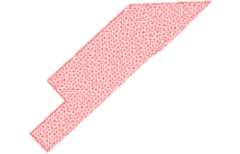
The first step is to go ahead and make the TIN MODEL, using the original XYZ data file. There’s nothing new here, so I’ll skip the details. The resulting 2D model is shown in the graphic to the right.
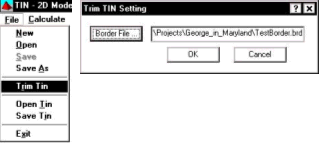
Now it’s time to cut the tin along our border. In the File Menu, you’ll find the latest addition in an item called ‘Trim Tin’. When you click it, you’ll be asked to supply a HYPACK® MAX Border (BRD) file.
The existing TIN is now trimmed to conform to the edges of the border file. Additional XYZ data points are created at every point where a triangle leg intersects
I can now use the remaining information and run volume computations on it using any of the methods available in the TIN MODEL program. For example, the report from the Philadelphia Method is shown in the text box below.
Philadelphia Pre-Dredge Report_sample
You can see that it only provides quantities in the areas contained in the polygon and 0.0s for lines that are outside the desired area.
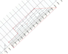
The same technique (TrimTin) can be used to isolate contours only in a user-desired area. In the graphic to the right, I generated contours inside the polygon area by first, making the model; second, trimming the tin to a border file; third, exporting DXF contours from the TIN MODEL on the trimmed model.
Qフィラデルフィア法体積計算2(Explanation of Philadelphia Volume Summaries)[英語]
FAQ ID:Q13-18
I recently was asked by a user what all of the different items that were included in the Philadelphia Post-Dredge Volume Summary meant. It took me a couple of minutes to figure it out, even though I work with it about every other week. I figured it would be good to run a test example and explain some of the output.
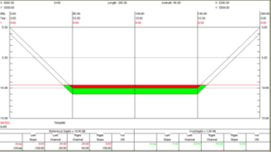
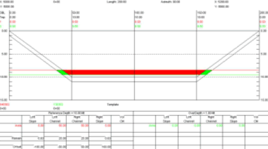
Step 1: 8.5m Data Set in Philadelphia Pre-Dredge
I first created two test data sets that would create a set of data at 8.5m and 9.5m across my survey lines.
My first data set and the associated cross section template are shown in the figure to the right.
The template points are as follows:
| Distance | Depth |
|---|---|
| 0.0 | 0.0 |
| 50.0 | 10.0 |
| 100.0 | 10.0 (Centerline) |
| 150.0 | 10.0 |
| 200.0 | 0.0 |
All of the depths in the first data set are at 8.5m. There are ten parallel lines.
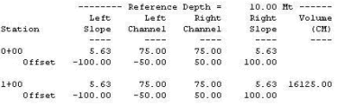
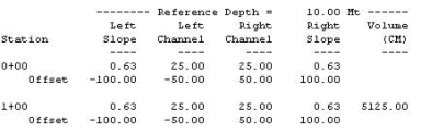
I first ran the volumes for this data set using the Philadelphia Pre-Dredge method. This generated the report shown to the right:

The Left Slope and Right Slope areas are reported as 5.63 m2each. This is correct as shown in the figure below.
The area for the Left Channel and Right Channel is simply the height times width (1.5 x 50) and the 75 m2 shown in the report is correct.
Since each section is identical, the volume is equal to the sum of the area under each section (161.25² ) multiplied by the distance between sections (100) giving 16125.00 m³.
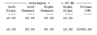
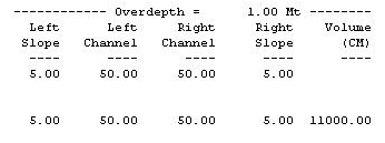
The overdepth template was placed one meter below the design template. The results from the volume report are shown in the figure right.
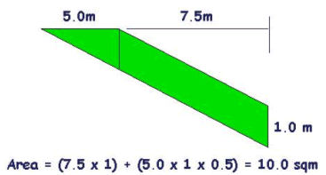
The left slope area is identical to the right slope area and is shown in the figure below. The volume is shown to be 10m², which is identical to that shown in the CROSS SECTIONS report.
The overdepth in the Left Channel and Right Channel is equal to the depth of overdepth template beneath the design template (1.0m) times the distance (50m) which is 50m².
The area between two sections is equal to the average area under a section (120m; they are identical sections) times the distance between sections (100) resulting in 12,000 m³ which is the volume shown in the report.
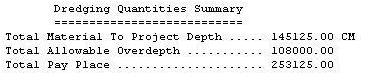
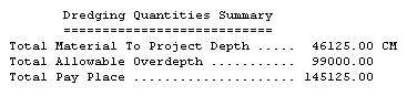
The results for the channel (nine pairs of lines) are shown in the figure to the right.
The Total Material To Project Depth is total volume of material located above the design template. This is equal to our area per section above the design template (16,125 m³) times the number of pairs of lines (9) and is exactly correct.
The Total Allowable Overdepth is the total amount of material located between the design and overdepth templates. This is equal to our volume per section (12,000 m³) times the number of line pairs (9) = 108,000 m³. Once again, the CROSS SECTIONS program is exactly correct.
The Total Pay Place is simply the sum of the two items above.
Step 2: 9.5m Data Set in Philadelphia Pre-Dredge
I next created a new data set, using the same template, but changing all of the depths to 9.5m. A typical section is shown in the figure right.
The design material is shown in the figure right. I’ll leave it to you to prove the areas and volumes are correct. [Trust me, they are.]
The overdepth material is shown in the figure right. Once again, feel free to verify that the areas and volumes are correct. [They are.]
Finally, the volume summary from the Philadelphia Pre-Dredge report is shown in the figure to the right. All values are correct and now we are ready for the BIG test.
Step 3: 8.5m and 9.5m Datasets in Philadelphia Post-Dredge Method.
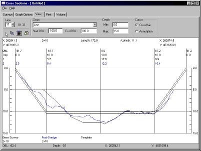
Finally, I entered both the 8.5m dataset (PreDredge) and my 9.5m dataset (PostDredge) datasets into the Philadelphia Post-Dredge Method and examined the results. A typical cross section is shown in the figure right.
Notice that the program now colors the material removed, not the material remaining. This is something that confuses a lot of users.
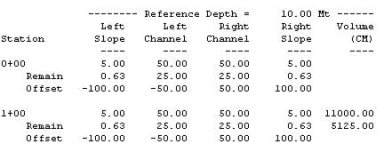
The results for the first two sections are shown in the figure to the right.
The “Area” shown in the report is the area of material removed in that section. Note that it is possible to get a negative area for a segment if the area computed from your post-dredge survey is greater than the area from your pre-dredge survey.
| Left Slope | Left Channel | Right Channel | Right Slope | |
|---|---|---|---|---|
| 8.5m Area | 5.63 m² | 75.00 m² | 75.00 m² | 5.63 m² |
| 9.5m Area | 0.63 m² | 50.00 m² | 50.00 m² | 0.63 m² |
| Material Removed | 5.00 m² | 25.00 m² | 25.00 m² | 5.00 m² |
The Remain areas are generated from the 9.5m data set and are identical to those computed when we ran the Philadelphia Pre-Dredge volumes for that data set.
The volume for the first section (11,000 m³) is the same value achieved by taking the volume for the 8.5m data set (16,125 m³) and subtracting the volume from the 9.5m data set (5,125 m³). The same is true for the Overdepth areas and volumes.
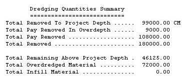
The summary for the Philadelphia Post-Dredge Volume Report is shown above. The values are explained as follows:
Total Removed To Project Depth: This is the difference between the volume (above design template) computed for the Pre-Dredge data set (145,125 m³) minus the volume computed for the Post-Dredge data set (46,125 m³). Note that this can be a negative number if there is more material present in the Post-Dredge survey!
Total Pay Removed in Overdepth: This is the difference between the volume of material contained in the area between the design and overdepth templates for the Pre-Dredge data set (108,000 m³) minus the volume for the same area in the Post-Dredge data set (99,000 m³).
Total Pay Removed: This is the sum of the Total Removed to Project Depth and the Total Pay Removed in Overdepth.
Total Removed: This is the total material difference between the Pre-Dredge survey and the Post-Dredge survey without regard to the design and overdepth template. In our example, the survey area covered a 200m x 900m area (180,000 m²). We changed the surface from 8.5m to 9.5m, taking away 1m of material. Multiplying the area (180,000 m²) by the height (1m) gives us 180,000 m³, representing the Total Removed.
Total Remaining Above Project Depth: This is the remaining material above the design template from our Post-Dredge survey. It is independent from the Pre-Dredge survey surface and represents how much material you have to remove to get the channel down to the project design.
Total Overdredged Material: This represents the material that has been removed beneath the overdepth template. It is computed by taking the Total Removed (180,000 m³) and subtracting from it the Total Pay Removed (108,000 m³). In our example, this results in an answer of 72,000 m³.
Total Infill Material: This is the volume of material where the Post-Dredge survey is deeper than the Pre-Dredge survey. In our example, we have no such area and the result is 0.00 m³.
Qシングルビームデータと体積計算について(The Effect of "Along-Line" Spacing of Soundings in Single Beam Data on the Computation of Average End Area Volumes)[英語]tion of Average End Area Volumes
FAQ ID:Q13-19
Well, that's a hell of an impressive title. If I were to tell you of a way that you could make $20,000 without any additional effort would you be interested? If I tell you how, would you give me half? If your answer to the last two questions is "Yes", then read on. Otherwise, go look at the cartoon.
HYPACK® can collect every sounding that comes out of your echosounder. If your sounder is updating at 15 times per second and your boat is traveling at six knots, this means you will have a sounding every 8" along your planned line.
Now, when you go to compute volumes, should you use all of these soundings or should you "thin" the data by using one of the sounding selection programs?
In preparation for my Volume Seminar at the 2001 U.S. Hydrographic Conference (21-24 May 2001 - Sheraton Norfolk Waterside Hotel - details at www.thsoa.org) I took a single beam data set and did some tests to determine how the volumes compared when I thinned the data using different spacings.
Below is a plot, taken from a capture of the CROSS SECTIONS program. The original survey data is spaced about every 8" and is in black. I then ran the data through the MAPPER program, using a 20' x 20' matrix and saved the point "Closest to the Center" of each cell to an XYZ file. [It's a little more complex, as I then took the XYZ file result from MAPPER, ran it into the TIN MODEL and then cut sections through it to get it back into EDITED ALL format so I could then load the results back into CROSS SECTIONS.] The soundings at 20' spacing are shown in red on the picture below.
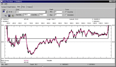
Visually, there isn't a whole lot of difference between the two sections. The file with the 8" spacing moves above and below the file with the 20' spacing, but it's not evident what the effect will be on the volumes.
I ran volume quantities for the entire channel, once for the 8" data and again for the 20' data. The 8" data had almost 3% more material. I then ran some more tests, sampling the data at 2', 5', 10', 20' and 50' spacing to see the result. The computed volumes are summarized in the table and graph below.
| Spacing | Dredge Material (cubic yards) |
% of original |
|---|---|---|
| 8" | 28,938 | 100 |
| 2' | 28,911 | 99.9 |
| 5' | 28,782 | 99.5 |
| 10' | 28,009 | 96.8 |
| 20' | 28,151 | 97.3 |
| 50' | 28,630 | 98.9 |
The test conducted on this data set was repeated on a different data set with almost identical results.
So, if I want to maximize my volume quantities, I will use every data point in the sounding set. If I want to minimize my volume quantities, I will thin the data every 10' along the line.
The difference in this data set between those two approaches is 929 cubic yards. At $22/yard, that comes to a savings of $20,438.