HYPACKに関する質問
5.一般事項(HYPACK® Max General)に関するFAQ
Qカタログファイルの操作(Working with Catalog Files (*.LOG))
FAQ ID:Q5-1
新しいカタログファイルの作成
HypackMaxが自動で作成するものと異なるカタログファイルが必要となるかもしれません。その場合は以下のような手順で簡単に新しいカタログファイルが作成編集等が行なえます。
DataFileList 内のProjectDataフォルダで右クリックしてドロップダウンメニューから「CREATE NEW LOG FILE」を選択します。すると、データフォルダ内の全データファイルリストのダイアログが表示されます。
Creating a New Catalog File (Before)
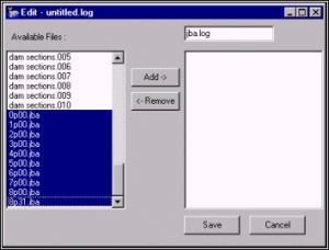
右上角のボックスに新しいログファイルの名前を入力します。
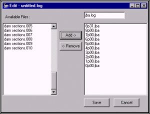
ログファイルに入れたいデータファイル名を選択し、「Add」ボタンをクリックします。HYPACK MAXは最初に選んだフォルダ(Raw・Edit・Sort)に、この作成されたファイルを拡張子LOGで保存します。
Creating a New Catalog File (After)

カタログファイルの編集
The Edit Log File Dialog
DataFileList 内のProjectDataフォルダで右クリックしてドロップダウンメニューから「EDIT NEW LOG FILE」を選択します。すると、カタログ内のファイルのリストとプロジェクト内で操作できるその他のファイルのダイアログが表示されます。
カタログ内のファイルリストから選択して「Remove」をクリックすることによってリストから測量ファイルを削除できます。
操作可能な測量ファイルを選択し、「Add」をクリックすることによってファイルをリストに加えることができます。
カタログファイルの合成(現在、使用不可)
データファイル内のカタログファイルまたはデータファイルフォルダで右クリックすると、メニューに一組の合成機能のリストが現れます。現在の時点ではこの機能は正常に働きません。従って、この機能で新規にファイルは作成しないでください。
Q緯度経度表示への切替と入力機能(Changes to Lat-Long Display and Input Functions)
FAQ ID:Q5-2
HYPACKR MAX には、X-Y座標からローカルの緯度経度へ、さらにWGS-84の緯度経度に変換する手順が幾つか有ります。我々は何人かの顧客との長い議論の末に、 WGS-84以外のローカル座標上に緯度経度を表示するために使われている多くの機能を変更しなくてはならないとの結論に達しました。これらの変更は、 バージョン00.5A CD以降のものに反映されています。これ以前のバージョンに対しては、Tech Supportサイトから最新版のHYPACK.EXEとDRAW32A.DLLをダウンロードする事でアップデート可能です。
以下の表示個所にこれらの変更が反映されています:
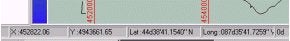
HYPACKR MAX スクリーン内のカーソル位置の緯度経度表示。
HYPACKR MAX スクリーンの画面下には、カーソル位置のX-Yや緯度経度が表示されている。前のMAXのバージョンでは、これはWGS-84の緯度経度が表示されている。DRAW32A.DLL をダウンロードして \HYPACK ディレクトリにコピーする事によってローカルの緯度経度で表示する事が可能になります。
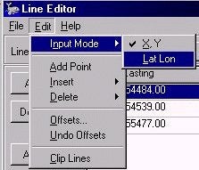
Line Editorプログラムでの緯度経度表示。
多数のユーザは、Line EditorでのWaypointをX-Y(Default)か緯度経度の何れかで入力可能であるという事に気づいていませ ん。00.5Aより古いバージョンでは、WGS-84の緯度経度で入力しなくていけませんでした。DRAW32A.DLLをダウンロードし¥HYPACK ディレクトリにコピーする事によって、ローカルに基づいた緯度経度の情報を入力する事ができるようになりました。
別の変更点としては、Input ModeがLat-Longに設定されている時は、分解能が向上します。00.5A以前のバージョンでは、DDD-MM.MMMM のフォーマットで緯度経度を入力しなければならなく十分な精度が得られませんでした。
図に示す様にフォーマットがDDD-MM-SS.SSSS に変更されました。この変更を反映させる為には、Tech Support ページから最新版のHYPACK.EXE をダウンロードし、それを\HYPACK ディレクトリにコピーします。
MAXとSURVEYでの緯度経度 グリッドの表示。5A以前のバージョンでは、MAX SURVEY画面に表示される緯度経度 グリッドはWGS-84のグリッドです。
DRAW32A.DLLをダウンロードする事によって、両方のプログラムでローカル座標での緯度経度 グリッド表示が可能となります。
Qカラー設定共通ダイアログ(Common Color Dialog)
Q後処理(ポストプロセス)のガイド(Post-Processing Guides)
FAQ ID:Q5-4
HypackMAXにはいくつかのデータ選択プログラム と最終成果作成プログラムがあるため、どのプログラムを使用すればよいかまようことがあるかも知れません。次のフローチャートは、シングルビームデータの処理手順を示します。
まず、全てのシングルビームデータに、音速度補正を適用するためにSOUND VELOCITYプログラムを実行する必要があります。それから、SINGLE BEAM EDITORで潮位補正を適用し、そして、悪いデータを削除します。出力されるファイルは編集済みのALLフォーマットファイルとなります。
その後の処理はいくつかの手順を選択することになります。
Sounding Selectionプログラム( SORT、MAPPER、CROSS SORT )は、結果の正確度に影響を及ぼすことなく最終成果作成の計算を加速するプログラムです。各々の概観は、この章に後半で理解できるでしょう。使用するプロ グラムの選択はどの方法を好むか、最終成果作成の際にどのフォーマットのファイルを必要としているかで決まります。
HYPLOT、TIN MODEL、及び、EXPORTは、XYZフォーマットかAllフォーマットのいずれかのファイルを使用します。従って、データを削減する場合、Sounding Selectionプログラムのうちのどれでも利用可能となります。
シングルビームRawデータのFinal Product(Hyplot、Tin Model、Export)までの流れ
CROSS SECTIONS AND VOLUMESプログラムは、Allフォーマットファイルにおいてのみ添付されるチャネルテンプレート情報を必要とします。CROSS SORTプログラムは、出力フォーマットにおいてこの情報を保持する唯一の測深データ削減プログラムです。従って、CROSS SECTIONS AND VOLUMESを使用する前にデータの削減を行う場合はCROSS SORTのみが使用可能となります。

マルチビーム後処理ガイド
次のフローチャートは、マルチビームデータ処理の概要を示します。
マルチ‐ビーム、多素子測深器データの全ては、まず、Multibeam Editor またはMB-MAXを使用して潮位補正を適用し、悪いデータを削除しなければなりません。その結果生じる出力データ形式は、XYZフォーマットファイルとなります。その後の処理にいくつかの選択肢があります。
Sounding Selectionプログラム( MAPPER、及び、SOUNDING REDUCTION )は、結果の正確度に影響を及ぼさずにあなたの最終成果物の計算を加速するデータ削減プログラムです。各々の概観は、この章に後半で理解できるでしょう。 使用するプログラムの選択はどの方法を好むか、最終成果作成の際にどのフォーマットのファイルを必要としているかで決まります。
マルチビームRawデータのFinal Product(Hyplot、Tin Model、Export)までの流れ
HYPLOT、TIN MODEL、及び、EXPORTは、XYZフォーマットかAllフォーマットのいずれかのファイルを使用します。従って、データを削減する場合、Sounding Selectionプログラムのうちのどれでも利用可能となります。
マルチビームRawデータのCross Sections and Volumesプログラムまでの流れ
CROSS SECTIONS AND VOLUMESは、その計算をするのにチャネルテンプレート情報を必要とします。XYZファイルはテンプレート情報を含まないので、Tin Modelプログラムに断面情報としての計画測線ファイルと共に読み込むことによって、ALLフォーマットに変換しなければなりません。
Qマウスの右ボタンに割り振られている機能
FAQ ID:Q5-5

マウスの左ボタンに休みを与えてあげて、右ボタンの機能を見てみましょう。そこにはHypack®Max 005aには無かった”Enable”機能がいくつかあります。例えば、MAX design screen上の"data files" の領域にあるRAWやSORT、 EDITED DATA FILESフォルダを右クリックすると旧バージョン8.9のFile Managerにあった機能の多くが表示されます。航跡と測深値をデスクトップ上に表示させたいときには、"enable tracklines"と"enable soundings"にチェックを付けます。(この機能を追加してほしいという声が多くありました。)
enableにチェックを入れた状態の LOG FILEを右クリックすると、"show lines report"と呼ばれる新しい機能が現れます。この機能は、データ収録中の実際の総距離を表示させる機能です。
もしも、XYZ fileが、SORT DATA FILES fileフォルダにあるならば、XYZ file上で右クリックしてみましょう。HYPACK BORDER EDITORで作成したファイルを利用して、望むままの大きさ・形状のXYZ fileを新たに作成することができるのです!
適用前
適用後
project filesの中にenableにチェックが入ったDXFファイルがあるなら、右クリックしてみましょう。EXPORT TO LNWメニューが現れます。これは、初めDXF2LNWと名づけられていたユーティリティです。
SURVEYプログラム中での右クリック機能の中でも二つの主要なものは、直にTARGETやBOAT (もしくはcrosshairs) 上でクリックした時に現れ、各々の表示方法を変更できる項目です。
TIN MODELでは、タイトルバーのメニュー領域から項目を選ぶより、右クリックで表示されるメニューから項目を選ぶほうが手間が省けます。
QHypackMaxショートカットガイド(Hypack Max Shortcut Guide)
FAQ ID:Q5-6
最近、あるユーザーと一緒に作業をしていましたが、その中であった質問の一つに、プログラムへのショートカットとは何か、というのがありました。プログラム中にはユーザーに解りやすいショートカットがいくつも用意してあります。
Surveyプログラムには、キーボードを使って操作できる機能がいくつもあります。現在、それらを全てリストにしようとしているところです。もし、書き漏らしがあってもご了承ください。
データ収録に関する操作
CTRL - S データ記録開始
CTRL - E データ記録終了
CTRL - U データ記録一時停止
CTRL - R データ記録再開
イベントマークやターゲットを入力
F-5 ターゲットの印をうつ
CTRL - N イベントマークを入れる
測線ファイル関連
CTRL - W 測線開始点を入れ替える(測線の方向)
CTRL - I 測線番号を次の測線番号へ増やす(次の測線へ)
CTRL - D 測線番号を前の測線番号へ減らす (前の測線へ)
CTRL - F 次の予定通過点(もしくは測線部分)へ移す
CTRL - B 前の予定通過点(もしくは測線部分)へ移す
リアルタイム潮位に関して
ALT - Y 潮位を増加させる
ALT - Z 潮位を減少させる
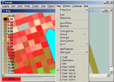
Survey programには、Mapに対するメニュー項目があります。電子海図をプロジェクトへ読み込みしているけど、Survey programで電子海図を表示させることができません。しかし、一旦プロジェクトから電子海図を外して、再び読み込ませると表示させられます。一旦外し て、再度読み込ませるという煩わしさを避けるには、Mapメニュー項目を選択して、表示させる電子海図を選択してください。Chartの文字の横にチェッ クマークが入っているときは、その項目が表示されています。チェックが入っていないときは、読み込まれているけれども表示されていない状態です。これは、 Mapメニューの下側にある項目全てについていえます。以下はメニューの表示例です。
Q測深データの点表示(Pixel Soundings Option in HYPACK Max)
FAQ ID:Q5-7
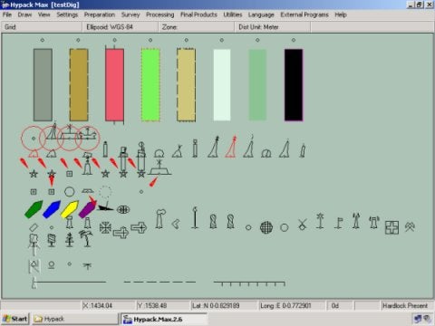
HypackMAXより測深点の点表示が可能になりました。 (Figure 1a).
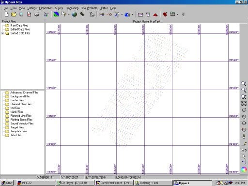
Figure 1a
測深点のサイズはユーザーにより設定可能で、視認し易いサイズで表示が可能です。 (Figure 1b).
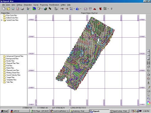
Figure 1b
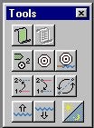
QSurveyプログラムの新しいインターフェイス(Dockable Toolbar in Survey)[英語]
FAQ ID:Q5-8
Survey program has new graphical user interface. When you start the latest Survey the toolbox is going to be attached to the menu bar.
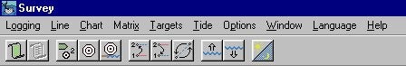
We hope he meaning of each button is self-explanatory. In case you can not guess, hold your cursor on the button and a tool tip will define the function. (The function of each is described here in the legend to the left). The toolbox can be placed anywhere on your screen (even outside of Survey window). You just have to point your mouse to the edge of the toolbox and drag it to desired position. If you place the toolbox close to Survey window edge, it will attached. The toolbox window can be closed and/or resized.
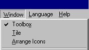
There is a menu item Windows/Toolbox that closes/restores the toolbox.
QDGW、DIGファイルの出力(Plotting .dgw and .dig Symbols)[英語]
FAQ ID:Q5-9
When plotting symbols, it readily becomes apparent that HYPACK® has not always done as good of a job as it might. This problem arises when using a single set of bitmap fonts for display on all devices. What looks nice and readable on the screen becomes a smudge or dot on a high resolution plotter. One customer asked us to send him the corresponding True type fonts for our symbols. Great idea! ... but no, we don't use them and don't want to spend the time in one of those awful editors. Our solution is in line with the IHO S52 symbol library, which we use to display S57 data with, and that is HPGL style code. This is a vector drawing language which can be scaled and displayed exactly on all devices at any resolution. Below is a screen capture of the new .dgw symbols. We have another for the .dig symbols and added a new option to display the text associated with the .dig objects.
QSurveyプログラムの各種表示方法の設定について(Survey Schemes and the The New Schemebuilder Program)[英語]
FAQ ID:Q5-10
What is a Scheme
In the newest version of HYPACK® Max, 02.6, coming out soon, Coastal Oceanographics, Inc. has developed the concept of "schemes" for the Survey program. Using schemes the HYPACK® Survey user has the ability to set color and font preferences for most of the screen objects in the Survey program, including the user interface colors for Windows®. The idea of schemes came about with the request of better day/night colors. Rather than setting colors we think the user might prefer for the night colors, schemes give the user the ability to set, and save, as many different color combinations as they prefer. Below is a screenshot of the Schemebuilder program.
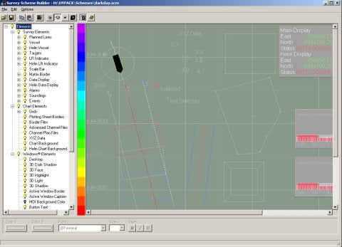
Image 1 - Schemebuilder program.
Using Schemebuilder
Launch Schemebuilder by clicking on the Settings->Schemebuilder menu item in HYPACK® Max. Using the program is very straight-forward. On the left you will notice a group of three different types of elements listed: Survey Elements, Chart Elements, and Windows® Elements. Survey elements are objects inside the program itself like the vessel colors, alarms, scale bar, etc. Chart elements are chart data types being drawn by Max's shared drawing engine. Windows elements are the colors of the user interface to your Windows® system (windows, desktop, etc.). When you click on one of the sub-items in the group its current color and/or font will be specified in the area below the window. You change the colors and/or font by selecting the new choice from a color/font dialog.
When you have specified the colors you would like for that scheme, you can then save the scheme into a .scm file. There a new directory under the HYPACK® Max root directory called 'Schemes' where the program will automatically attempt to save/open schemes from.
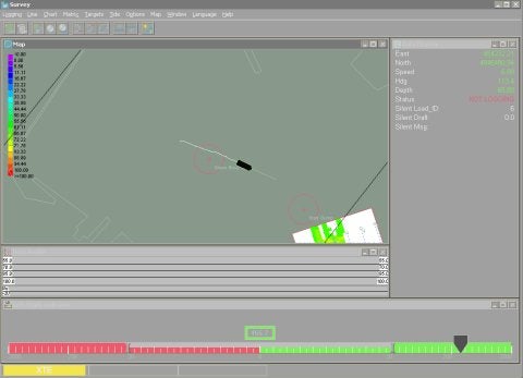
Image 2 - Survey program with the above scheme loaded.
Bring the Scheme into Survey
When running the Survey program, you can load a scheme by selecting the Options->Color Scheme... menu items. An open file dialog will appear with the directory set to the Schemes directory. Choose the scheme you prefer and it will become the default, meaning that it will load every time you run Survey thereafter (until otherwise specified).
QGeoTiFファイルを作成するユーティリティー(Freeware Program for Geo-referencing TIF Files)
FAQ ID:Q5-11
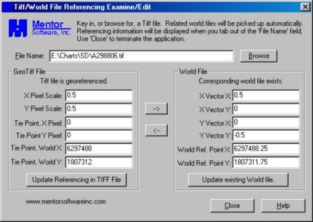
HypackではバックグランドデータとしてGeoTiffファイルの読み込みが可能となっています。この機能によ り航空写真などの画像ファイルを海図のように使用することが可能になります。GeoTiffファイルはTiffフォーマットのファイルに座標関連付けをす るTFWファイルを画像ファイルと同じフォルダに保存することで利用可能となります。
TFWファイルの内容は以下のようになっています。
- Xスケール (1ピクセルと実距離の比)
- Hypackでは未使用のフィールド
- Yスケール (1ピクセルと実距離の比)
- X基準座標
- Y基準座標
------------------実例---------------
1.50000000000000
0.00000000000000
0.00000000000000
-1.50000000000000
1934001.50000000000000
1187698.50000000000000
--------------------------------------
上例は画像ファイルのサイズが2000 X 2000、“x”基準座標が1934001.5でXスケールが1.5なので終点座標は基準座標から2000 * 1.5を加算した1937001.5となります。“y”基準座標は1187698.5なので 終点座標は2000 * -1.5を加算した1184698.5となります。
尚、GeoTiffファイルを作成するフリーウェアユーティリティプログラムが以下のWebサイトからダウンロードできます。
Mentor Software (http://www.mentorsoftwareinc.com) →サイトが閉鎖されました。
Q外部プログラム起動ユーティリティー(Launching External Programs from the Hypack® Max Menu)[英語]
FAQ ID:Q5-12
You can use the EXTERNAL PROGRAMS menu that will launch external executable files. Just another handy alternative to using the usual Windows® methods.
- Select EXTERNAL PROGRAMS-SETUP. The Tool Options dialog will appear.
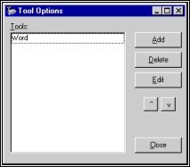
Tool Options dialog
- Click [Add] and the Tool Options Properties dialog will appear.
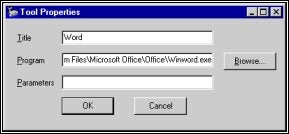
Tool Options Properties dialog
- Fill in the fields of the dialog then click [OK] and close the program.
The contents of the Title field will now appear in the Hypack® Max Help menu. In the future, when you select this menu item, it will launch the Program named in the second field and pass it any Parameters that you have listed.
The Current Project checkbox (not pictured here) is for internal use at Coastal Oceanographics Inc. only.
You can add as many programs as you want in this manner and use the up and down arrow buttons to arrange their order if desired.
To remove programs from the menu:
Open the Tool Options dialog, select the program to be removed and click [Delete].
To change the properties of any listed program:
Open the Tool Options dialog, select the program then click [Edit]. The Tool Options Properties dialog will appear with the current data and you can edit it as desired.
QS-57電子海図について[英語]
FAQ ID:Q5-13
One of the many changes in the hydrographic field over the past ten years is the use of S-57 for the storage, presentation and transfer of digital chart data. Coastal Oceanographics has been working for several years to be able to present S-57 format files in our HYPACK® MAX and other packages. As a result of this work, we have developed a product to create, maintain and update S-57 chart data.
S-57 is shorthand for Special Publication No. 57, “IHO Transfer Standard for Digital Hydrographic Data”. IHO is the acronym for the International Hydrographic Organization.
The purpose of this document is to provide you with a simple and straight-forward overview of the S-57 format. In other words, this document is sort of like an ‘S-57 for Dummies’ where the intent is to de-mystify how data is stored and managed.
A. Feature and Spatial Data
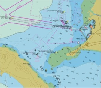
An S-57 file contains digital chart information that is divided into feature and spatial data. A feature is some kind of object, such as a buoy, or a rock, or a traffic separation zone or a light or one of several hundred available objects in S-57. There are point objects (buoys, wrecks, lights, ….), polyline objects (pipelines, cables, roads, ….) and closed polygon objects (depth areas, anchorages, shoreline, …..).
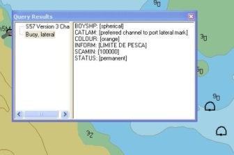
Each feature can be further described by a list of available attributes. For example, the lateral buoy shown in the lower right of the figure contains the following attribute information:
BOYSHP: [spherical]
CATLAM: [preferred channel to port lateral mark]
COLOUR: [orange]
INFORM: [LIMITE DE PESCA]
SCAMIN: [100000]
STATUS: [permanent]
Each attribute is described by a six-letter abbreviation. Thus, BOYSHP = Buoy Shape, SCAMIN = Scale Minimum. Each attribute can require a user entry, a single user choice from a list, or multiple user choices from a list.
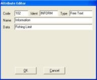
For example: The window to the right is the Attribute Editor for the INFORM attribute. It allows you to enter a single line of text. In this case, we have entered ‘Fishing Limit’.
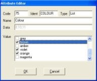
2nd Example: The window to the right is the Attribute Editor for the COLOUR attribute. Note that we can select a single color or multiple colors to describe the object. [In this example, we have the famous brown, violet and orange buoy, used to denote islands inhabited by people with no sense of color coordination.]
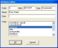
3rd Example: The window to the right is the Attribute Editor for the BOYSHP (Buoy Shape) attribute. In this case, we can only select one item from the available list.
So, a feature tells us what kind of object we have and there are attributes assigned to the feature to tell us some more details. We haven’t yet described where the object is located. That is done with the spatial data.
Spatial data is a fancy way of saying ‘where is the feature located’. In the S-57 format, the locations of objects are described by their WGS-84 positions. Although a user interface might allow you to enter and display the spatial data on a local coordinate system, deep in the bowels of the S-57 file, all the S-57 data is being written as a geographic coordinate (Latitude and Longitude) in WGS-84.
B. Nodes, Chains and Areas
It would have been simpler if they named these Points, Lines and Areas.
One of the favorite buzzwords of an S-57 jockey is ‘chain-node topography’. It’s a fancy way of saying that everything in your S-57 file is either a point (‘node’) or a series of lines (‘chains’). Sometimes the lines form an enclosed shape (‘area’).
A node is a single spatial data point, composed of a WGS-84 coordinate pair. There are two kinds of nodes, isolated and connected. An isolated node represents the position of a point feature, like a buoy or a rock or a wreck. It can’t be used for anything else.
A chain (also referred to by some as an ‘edge’) is a line or a polyline, constructed between two or more coordinate pairs. At each end of the edge is a connected node. We can connect one chain to another by either having them share the same connected node or by making another chain that connects their connecting node with a single line.
An area (also called a ‘face’ by some) is a series of chains (or a single chain) that starts and ends at the same connecting node. In other words, it’s a polygon that describes an area. An area can contain multiple chains (and contain multiple connecting nodes) or can be comprised of a single edge that starts and ends at a single connecting node.
At the top of the adjacent figure is CHAIN 1. This consists of a single line drawn between two connected nodes. This is the simplest of chains.
CHAIN 2 shows a series of coordinate pairs, terminated by connected nodes. This is more typical of an chain.
AREA 1 shows an area constructed from a single chain. It starts and ends on the same connected node.
AREA 2 shows an area constructed from four chains. It is very typical for a area to consist of multiple chains. You can also see another chain (CHAIN 3) taking off from a connected node. This is also very typical, as several features may share the same connecting nodes.
One of the things to keep in mind when you define an area is that as you move along a chain that bounds the area, the enclosed area is always off the right side of the chain.
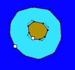
Take a look at the graphic to the right that shows an island (brown), surrounded by a Depth Area (0m to 5m in Light Blue), surrounded by a deeper depth area.
When we create the chain that describes the island as a ‘Land Area’, we need it to go counter-clockwise. That way, the area we are interested in defining is to the right as we traverse around the chain.
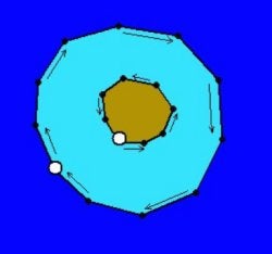
Now take a look at the graphic used to define the Depth Area. We need to define an area with a hole in it. This is done by defining one polygon along the outside and a second polygon along the inside.
Note that the chain defining the outside goes in a clockwise direction, keeping the Depth Area to the right. The chain surrounding the hole (island) travels in a counter-clockwise direction, meaning the depth area is to the right.
Luckily, we can use the same chain to define the Land Area and the inside of the Depth Area. When I select a chain to be used in the definition of an area, I can ‘reverse’ the direction of the chain when used by a particular feature.
C. Combining Features and Spatial Data
The S-57 format stores feature and spatial data as separate records. Each feature record contains information as to what spatial record(s) applies to the feature.
When I want a new buoy to be included in my S-57 file, I first create the buoy ‘feature’ and specify the attributes for the buoy. I then give it the position where I want it to place the buoy. A new feature record will be created that contains the feature type and attribute info. A new spatial record will be created that contains the coordinate point (as an isolated node).
When drawing the S-57 data, it comes across the new buoy in the feature records. It figures out what kind of buoy to draw and what labels are drawn with it from the attribute information in the feature record. The same feature record also contains the location of the spatial record that tells me where to draw the buoy. I open up the spatial record, get the coordinate pair for the buoy and then draw the feature at that location.
This seems a little crazy. Why not just keep the spatial data with each feature record?
One reason for the separation of feature and spatial data is that the same chain might be used for several different features. In our previous example with the island and the depth area, the same chain is used to create the Land Area and the Depth Area. Rather than listing the same set of points for each feature, we save space by only listing the points in one place.
Also, by using this approach, if we change a coordinate pair in the chain used to define the Land Area, we are also automatically changing the coordinate pair used in defining the Depth Area. If each feature had its own set of separate coordinate lists, we would have to make sure that we changed the coordinate pair in every feature’s coordinate list, instead of changing it in only one location in the S-57 scheme.
D. Boundaries and Clipping
S-57 files are ‘bounded’ by two parallels of latitude and two parallels of longitude. The area formed by the bounds is sometimes referred to as the ‘bounding rectangle’. It’s illegal to have any spatial data located outside the boundary area.
In the graphic shown, the top chain would be ‘illegal’, because it contains coordinate pairs that are outside the bounding rectangle.
The lower series of chains forms a legal area. We created it with ‘connected nodes’ along the boundary line, as other features may want to take off from these points.
Some S57 Editors will either automatically clip your chains that pass outside the bounding rectangle while others will just notify you that you have an illegal chain.
QDesignプログラムで作成した測線(LNW)をSurveyプログラム上で読み込んでいるのですが現在の船の位置よりかなり離れた場所に表示されます。何が間違っているのでしょうか?(下図参照)
FAQ ID:q6-2
- 測線(LNW)を作成する時のXY座標の入力は合っていますか?
HYPACKでは、南北が"Y"、東西が"X"の数学座標を使用しています。(下図参照)
- 測線(LNW)を作成した時の測地の設定(Geodetic Parameter)とSurveyで使用している測地の設定は一致していますか?もし異なっているようであれば、正しい測地系の設定に変更してください。
Q5:SurveyプログラムのWindowメニューでTSSのデータを確認すると正しく来ているのに画面下に"Heave"と赤く表示されるのはなぜでしょう?
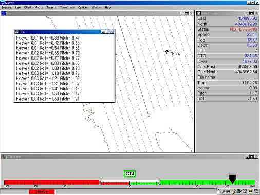
A5:HYPACKを終了し、DMSView又はターミナルソフトを使用してTSSからのデータ見て下さい。
データ中に含まれているフラグが小文字になっていませんか?(下図参照)
これは、何らかの原因でセルフテスト実行中である事が考えられるので大文字の"U"になった後に測量(Survey)を開始して下さい。
023DE7-0007u 00230038
023DF6-0007u 00160041
053E1C-0007u 00090044